Basic Graph Algorithms

参考：

• Chapter 5: Basic Graph Algorithms
• Chapter 6: Depth-First Search
• Wikipedia: Glossary of graph theory
• CS 137 - Graph Theory - Lecture 2
• COMPSCI 330: Design and Analysis of Algorithms - Lecture #5
• DFS Edge Classification
• Lecture 8: DFS and Topological Sort
• Lecture 21: Shortest Paths
• Lecture 20: Minimum Spanning Trees
• Math 575 - Problem Set 9

---

1. Definition

1.1 Simple Graph

Definition: Graphs without loops and parallel edges are often called simple graphs.

• loop: an edge from a vertex to itself
• parallel edges: multiple edges with the same endpoints
  • 注意 endpoint 表示的是 端点，并不一定是终点 (ending point)，也可以是起点

Non-simple graphs are sometimes called multigraphs.

Despite the formal definitional gap, most algorithms for simple graphs extend to non-simple graphs with little or no modification.

The definition of a graph as a pair of sets, $(V, E)$ forbids graphs with loops and/or parallel edges. 也就是说，用 $(V, E)$ 表示的图都 默认 是 simple graph.

We may (informally) use $V$ to denote the number of vertices in a graph (i.e. $\vert V \vert$), and $E$ to denote the number of edges (i.e. $\vert E \vert$). Thus, in any undirected graph we have $0 \le E \le {V \choose 2}$ and in any directed graph we have $0 \le E \le V(V − 1)$.

In this note we use the following terms:

• “Graph”, which generally means an undirected graph
• “Digraph”, which is used for directed graphs specifically

1.2 Neighbor and Degree

In this note we use the following notations for edges:

• $\lbrace u, v \rbrace$ can be a directed or undirected edge
• $u \to v$ represents a directed edge only

Definition: If there is an edge $\lbrace u, v \rbrace$, then $u$ and $v$ are neighbors mutually.

• For a undirected graph:
  • $\operatorname{degree}(u)$ == of $u$’s neighbors
• For a digraph:
  • If there is an edge $u \to v$, then
    • $u$ is a predecessor of $v$
    • $v$ is a successor of $u$
  • $\operatorname{in-degree}(u)$ == of $u$’s predecessors
  • $\operatorname{out-degree}(u)$ == of $u$’s successors

注意 predecessor 这个词并没有对应的动词。

1.3 Subgraph

Definition: A graph $G’ = (V’, E’)$ is a subgraph of $G = (V, E)$ if $V’ \subseteq V$ and $E’ \subseteq E$.

1.4 Walk, Path, and Cycle

Definition: A walk is a sequence of vertices, $\overline{v_1 v_2 \dots v_k}$, s.t. $\forall 1 \le i \le k$, $\lbrace v_i, v_{i+1} \rbrace \in E$.

• $v_1$ and $v_k$ are the endpoints of the walk
• $v_2, v_3, \dots, v_{k-1}$ are internal vertices
• The length of a walk is the number of edges, thus $k-1$.

A walk can consist of only a single node, with length $0$.

Definition: A walk is closed if $v_k = v_1$, and open if $v_k \neq v_1$.

Definition: A path is a walk that does not repeat vertices.

• So by definition, a path must be an open walk.

Definition: A cycle is a closed walk that does not repeat vertices except the endpoints.

• A cycle has at least 1 edge; it is not allowed to have a length of $0$.

Cycles of $n$ vertices are often denoted by $C_n$. (你把 $C_n$ 的 $n$ 理解为有 $n$ 条 edge 或是 length 为 $n$ 也是可以的). E.g.

• $C_1$ is a loop
• $C_2$ is a digon (a pair of parallel undirected edges in a multigraph, or a pair of antiparallel edges in a digraph)
• $C_3$ is a triangle.

1.5 Connectivity and Component

Definition: A graph $G$ is connected if $\forall$ 2 verices of $G$, $\exists$ a path between them. (其实你定义为 $\exists$ a walk 也是可以的，因为 $\forall$ 2 verices 一定是不同的两点，所以 walk 会升级为 path，不影响大局) Otherwise, $G$ is disconnected and it decomposes into connected components.

Definition: A graph $G$’s components are its maximal connected subgraphs.

• By “maximal”, it means you cannot add any element to $(V’, E’)$ of the subgraph $G’$ while keeping it connected.
• So the term “connected components” is actually redundant; components are connected by definition.
• Two vertices are in the same component $\iff$ there is a path between them.

Practically, the definition of component is only suitable for undirected graphs.

Definition: A digraph is strongly connected if $\forall$ 2 verices of $G$, $\exists$ a directed path between them.

1.6 Acyclicity

Definition: An undirected graph is acyclic if it contains no cycles, i.e. amongst all its subgraphs, none is a cycle. Undirected acyclic graphs are also called forests.

注意 forest 不一定就是 disconnected 的，有可能 disconnected 有可能 connected

Definition: A tree is a undirected, connected acyclic graph, or equivalently, one component of a forest.

Definition: A spanning tree of a graph $G$ is a subgraph that is a tree and contains every vertex of $G$.

Lemma: A graph has a spanning tree $\iff$ it is connected.

Definition: A spanning forest of $G$ is a collection of spanning trees, one for each connected component of $G$.

Definition: A digraph is acyclic if it does not contain a directed cycle. Directed acyclic graphs are often called DAGs.

Any vertex in a DAG that has no incoming vertices is called a source; any vertex with no outgoing edges is called a sink. Every DAG has at least one source and one sink, but may have more than one of each. For example, in the graph with only vertices but no edges, every vertex is a source and every vertex is a sink.

2. Traversing Connected Graphs / DFS / BFS

To keep things simple, we’ll consider only undirected graphs here, although the algorithms also work for directed graphs with minimal changes.

The simplest graph-traversal algorithm is DFS, depth-first search. This algorithm can be written either recursively or iteratively. It’s exactly the same algorithm either way; the only difference is that we can actually see the “recursion” stack in the non-recursive version.

# v: a source vertex
def RecursiveDFS(v):
	if v is unmarked:
		mark v
		for each edge {v,w}:
			RecursiveDFS(w)

# s: a source vertex
def IterativeDFS(s):
	PUSH(s)
	while the stack is not empty:
		v <- POP
		if v is unmarked:
			mark v
			for each edge {v,w}:
				PUSH(w)

N.B. IterativeDFS 最后一个 for 可以稍微改良一下：

# s: a source vertex
def IterativeDFS(s):
	PUSH(s)
	while the stack is not empty:
		v <- POP
		if v is unmarked:
			mark v
			for each edge {v,w}:
				if w is not visited:
					PUSH(w)

The generic graph traversal algorithm stores a set of candidate edges in some data structure that I’ll call a “bag”. The only important properties of a bag are that we can put stuff into it and then later take stuff back out. A stack is a particular type of bag, but certainly not the only one.

N.B. If you replace the stack above with a queue, you will get BFS, breadth-first search. And the breadth-first spanning tree formed by the parent edges contains shortest paths from the start vertex s to every other vertex in its connected component.

另外一个需要注意的是，还有一种改良方法是：stack 存储 (v, parent(v))。这么做并不是为了提升效率，而是为了方便遍历后迅速定位 path.

# s: a source vertex
def Traverse(s):
	put (None, s) in bag  # source vertex 的 parent 是空集
	while the bag is not empty:
		take (p, v) from the bag
		if v is unmarked:
			mark v
			parent(v) <- p
			for each edge {v,w}:
				put (v, w) into the bag

For any node v, the path of parent edges (v, parent(v), parent(parent(v)), . . .) eventually leads back to s.

If $G$ is not connected, then Traverse(s) only visits the nodes in the connected component of the start vertex s. If we want to visit all the nodes in every component, run Traverse on every node. (Let’s call it TraverseAll.) Since Traverse computes a spanning tree of one component, TraverseAll computes a spanning forest of $G$.

3. BFS/DFS 与 Spanning Tree

首先补充两个概念。Graph 里我们说 predecessor 和 successor，Tree 里面我们用 ancestor 和 descendant；不仅如此，我们还有 proper ancestor 和 proper descendant.

Suppose $T$ is a rooted tree with root $r$; $a$ and $b$ are 2 nodes of $T$.

Definition: If $a$ is in the path $\overline{b \dots r}$, then:

• $a$ is an ancestor of $b$
  • $b$ could be the ancestor of $b$ itself
• $b$ is an descendant of $a$
  • $a$ could be the descendant of $a$ itself.
• $a$ is a proper ancestor of $b$ if $a$ is an ancestor of $b$ and $a$ is not $b$ itself.
• $b$ is a proper descendant of $a$ if $b$ is an descendant of $a$ and $b$ is not $a$ itself.

Both DFS and BFS can generate spanning trees from graphs.

Suppose $G$ is a connected undirected graph, $T$ is a depth-first spanning tree computed by calling RecursiveDFS(s) where s is the root of the $T$.

Lemma 1. For any node v, the vertices that are marked during the execution of RecursiveDFS(v) are the proper descendants of v in $T$.

Lemma 2. For every edge {v,w} in $G$, either v is an ancestor of w in $T$, or v is a descendant of w in $T$.

Proof: Assume without loss of generality that v is marked before w. Then w is unmarked when RecursiveDFS(v) is invoked, but marked when RecursiveDFS(v) returns, so the previous lemma implies that w is a proper descendant of v in $T$. $\blacksquare$

4. Preorder and Postorder Labeling

def PrePostLabel(G):
	for all vertices v:
		unmark v
	
	clock <- 0
	
	for all vertices v:
		if v is unmarked:
			clock <- LabelComponent(v, clock)
			
def LabelComponent(v, clock):
	mark v
	
	prev(v) <- clock
	clock <- clock + 1
	
	for each edge {v,w}:
		if w is unmarked:
			clock <- LabelComponent(w, clock)
	
	post(v) <- clock
	clock <- clock + 1
	
	return clock

举个例子，假设有个 triangle abc，按 a → b → c 执行的情况应该是这样的：

mark a √
prev(a) = 0;
	mark b √
	prev(b) = 1;
		mark c √
		prev(c) = 2;
		post(c) = 3;
	post(b) = 4;
post(a) = 5;

return 6;

	a	b	c
prev	0	1	2
post	5	4	3

其实这里我觉得把 prev(a) 看做 “start time of accessing a” 或者 “time before accessing a”、把 post(a) 看做 “finish time of accessing a” 或者 “time after accessing a” 更好理解一点。

Consider $a$ and $b$, where $b$ is marked after $a$. Then we must have prev(a) < prev(b). Moreover, Lemma 1 implies that if $b$ is a descendant of $a$, then post(a) > post(b), and otherwise (“otherwise” 并不是是指 “$b$ is an ancestor of $a$”，而是指 “$b$ is not a descendant of $a$”，再结合 “$b$ is marked after $a$” 这个事实，只有一种可能是 “$a$ 和 $b$ 属于不同的 components”), prev(b) > post(a) (此时 $a$ component 遍历完了才轮到 $b$，prev(b) 的赋值必定在 post(a) 之后)。

Thus, for any two vertices $a$ and $b$, the intervals [prev(a), post(a)] and [prev(b), post(b)] are either disjoint or nested; in particular, if edge $\lbrace a,b \rbrace$ exists, Lemma 2 implies that the intervals must be nested.

5. Acyclicity in Directed Graphs

Lemma 2 implies that any depth-first spanning tree $T$ divides the edges of $G$ into two classes:

1. tree edges, which appear in $T$, and
2. back(ward) edges, which connect some node in $T$ to one of its ancestors.

其实这里可以进一步细分。考虑到 $T \subseteq G$ ($T$ 是 $G$ 的 subgraph)，这样至少有两个部分：$T$ 和 $G \setminus T$。

We call an edge $a \to b$ exists in $G$:

• if $a \to b$ is an edge in $T$, a tree edge.
  • 意思即是 $T$ 中所有的 edge 都叫 $G$ 的 tree edge
• if $a \to b$ is an edge in $G \setminus T$:
  • a forward edge if $a$ is an ancestor of $b$ in $T$
    • 注意 ancestor 是在 $T$ 中判断的，所以简单说就是在 $G \setminus T$ 是 $a \to b$ 且在 $T$ 中有 $a \to \dots \to b$
  • a back(ward) edge if $a$ is an descendant of $b$ in $T$
    • 注意 descendant 是在 $T$ 中判断的，所以简单说就是在 $G \setminus T$ 是 $a \to b$ 但在 $T$ 中是 $b \to \dots \to a$
    • 这样就发现了一个 cycle
  • a cross edge otherwise
    • 简单说就是在 $G \setminus T$ 是 $a \to b$ 但在 $T$ 中 $a$ 既不是 $b$ 的 ancestor 也不是 descendant

我觉得还是举个例子说明下比较好：

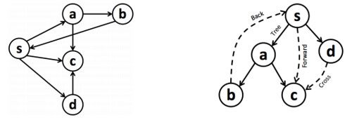
• 右图的实线是 $T$，所以实线的 edge 都是 tree edge
• 存在 $s \to c$ 属于 $G$ 但不属于 $T$，且在 $T$ 中 $s$ 是 $c$ 的 ancestor，所以 $s \to c$ 是 forward edge
• 存在 $b \to s$ 属于 $G$ 但不属于 $T$，且在 $T$ 中 $b$ 是 $s$ 的 descendant，所以 $b \to s$ 是 backward edge
• 存在 $d \to c$ 属于 $G$ 但不属于 $T$，且在 $T$ 中 $d$ 既不是 $c$ 的 ancestor 也不是 descendant，所以 $d \to c$ 是 cross edge

edge type of $a \to b$ in $G$	relationship of $a$ and $b$ in $T$	prev / post order
tree / forward	$a$ is an ancestor of $b$	prev(a) < prev(b) < post(b) < post(a)
back(ward)	$a$ is an descendant of $b$	prev(b) < prev(a) < post(a) < post(b)
cross	$a$ is neither an ancestor nor descendant of $b$	prev(a) < post(a) < prev(b) < post(b), 假设 $a$ 先访问到

obs: There is a backward edge in $G \setminus T$ $\iff$ $\exists$ a directed cycle in $G$.

除了这个算法外，书上还提供了一个在 DFS 的过程中 detect cycle 的算法：

def IsAcyclic(G):
	add a source vertex s
	for all vertices v ≠ s:
		add edge s → v
		status(v) <- New

	return IsAcyclicDFS(s)
	
def IsAcyclicDFS(v):
	status(v) <- Active
	for each edge v → w:
		if status(w) == Active:
			return False
		else if status(w) == New:
			if IsAcyclicDFS(w) == False
				return False
	status(v) <- Done
	return True

6. Topological Sort

A topological ordering of a digraph $G$ is a total order $\prec$ on the vertices such that $a \prec b$ for every edge $a \to b$. Less formally, a topological ordering arranges the vertices along a horizontal line so that all edges point from left to right.

A topological ordering is clearly impossible if the graph $G$ has a directed cycle – the rightmost vertex of the cycle would have an edge pointing to the left! On the other hand, every DAG has a topological order.

Idea: Run DFS on every vertex $x_i$ of $x_1,\dots,x_V$ and sort the vertices by $post(x_i)$ in reverse order.

Correctness of the Idea: By Lemma 2, for every edge $a \to b$ in a DAG, the finishing time of is $a$ greater than that of $b$, as there are NO back edges (because DAG has no cycle) and the remaining three classes of edges have this property.

Improvement: However actually you don’t need to sort. 我们看下 DFSAll 的写法：

def DFS(v):
	mark v
	
	prev(v) <- clock++
	
	for each edge v → w:
		if w is unmarked:
			parent(w) <- v
			DFS(w)
	
	post(v) <- clock++

def DFSAll(G):
	clock <- 0
	
	for each vertex v:
		if v is not marked
			DFS(v)

从最后的结果来看，finishing time, i.e. $post(x_i)$ 的顺序并不会因为 for each vertex v 的遍历顺序而改变。也就是说，DFSALL(G) 和 DFS(source) 从结果上来看本质是一样的，而且都是 $O(V+E)$.

考虑个简单的图 a → b → c：

• 假设 DFSAll(G) 的顺序是 c、$b$、$a$，得到的结果是 post(c)=1、post(b)=3、post(a)=5
• 假设 DFSAll(G) 的顺序是 b (所以包括了 c)、a，得到的结果是 post(c)=2、post(b)=3、post(a)=5
• 假设 DFSAll(G) 的顺序是 a (所以包括了 b 和 c)，得到的结果是 post(c)=3、post(b)=4、post(a)=5

所以你其实只用记录下 $post(x_i)$，然后根据它逆序排列 $x_i$ 就可以了。

RT: 所以 Topological Sort 的时间复杂度和 DFSAll 是一样的，都是 $O(V+E)$

7. Strongly Connected Components (SCC)

In a digraph $G = (V,E)$, vertex $a$ is connected to vertex $b$ if there exists a path $a \to b$.

In a digraph $G = (V,E)$, vertex $a$ is strongly connected to $b$ if there exists a path $a \to b$, and also a path $b \to a$.

If $a$ is strongly connected to $b$, we write $a \sim b$, and $\sim$ is an equivalence relation.

• Reflexivity: $a \sim a$, i.e. $a$ is strongly conneted to itself.
• Transitivity: if $a \sim b$ and $b \sim c$, then $a \sim c$.
• Symmetry: if $a \sim b$, then $b \sim a$.

In a digraph $G = (V,E)$, a Strongly Connected Component (SCC) is a maximal subgraph $S = (V_s, E_s)$ s.t. $\forall$ two vertices $a, b \in V_s$, $a \sim b$.

• 注意这里 maximal 并不是 SCC 的特殊要求，而是因为 component 本身就是 maximal subgraph
• Undirected graph 的 component 在平面上很好认，一定是一个独立且完整的 subgraph，比如一整段的 path 或是一整个 cycle
• SCC 则不同，独立的一整段 path 或是一个 cycle 可能只有一部分是 strongly connected 的，但是这一部分也符合 SCC 的定义，也可以是 SCC

We can see SCCs as equivalence classes of $~$.

For any digraph $G$, the strong component graph $scc(G)$ is another digraph obtained by contracting each strong component of $G$ to a single (meta-)vertex and collapsing parallel edges.

Let $C$ be any strong component of $G$ that is a sink in $scc(G)$; we call $C$ a sink component. Every vertex in $C$ can reach every other vertex in $C$, so a depth-first search from any vertex in $C$ visits every vertex in $C$. On the other hand, because $C$ is a sink component, there is no edge from $C$ to any other strong component, so a depth-first search starting in $C$ visits only vertices in $C$.

So we can come up with an idea to find all SCC in $G$:

• find a sink SCC, $C_{s1}$ of $G$, and remove it from $G$;
• find a sink SCC, $C_{s2}$ of $(G - C_{s1})$, and remove it;
• …
• till $G$ is empty.

所以问题转换为 “to find a sink SCC”。又因为，只要找到了一个 sink SCC 的 vertex，就能 DFS 得到 sink SCC，所以问题进一步转换为 “to find a vertex in a sink SCC”。

• Digress: How to find a SCC given a vertex $v$ in graph $G$, i.e. to find a SCC of $G$ containing $v$?
  • DFS(v,G) $\Rightarrow Reach(v,G) = \lbrace \text{vertices that } v \text{ can reach in } G \rbrace$
  • DFS(v,rev(G)) $\Rightarrow Reach^{-1}(v,G) = \lbrace \text{vertices that can reach } v \text{ in } G \rbrace$
  • Then $SCC(v,G) = Reach(v,G) \cap Reach^{-1}(v, G)$

Lemma 4. The vertex with largest finishing time (i.e. post(x)) lies in a source SCC of G.

Lemma 5. For any edge $a \to b$ in $G$, if post(a) < post(b), then $a$ and $b$ are strongly connected in $G$. (hint: backward edges)

It is easy to check that any directed $G$ has exactly the same strong components as its reversal $rev(G)$; in fact, we have $rev(scc(G)) = scc(rev(G))$. Thus, the vertex with the largest finishing time in $rev(G)$ lies in a source SCC of $rev(G)$, and therefore, lies in a sink SCC of $G$.

Actually you even don’t have to repeat the “find-remove” procedure. The Kosaraju algorithm could find all SCCs this way:

• Step 1: DFSAll(rev(G)) outputs vertices in the reverse (descendant) order of finishing time. Suppose the order is a → b ... → z:
  • source → sink order in $rev(G)$
    • i.e post(a) > post(b) > ... > post(z) in $rev(G)$.
  • sink → source order in $G$
    • i.e. post(a) < post(b) < ... < post(z) in $G$.
• Step 2: DFSAll(G) in the order above
  • Each call to DFS in the loop of DFSAll(G) visits exactly one strong component of $G$:
    • If $a$ cannot reach any vertex, then $a$ is an SCC itself.
      • Enter the next iteration in DFSALL(G) calling DFS.
    • If $a$ can reach a vertex i, because post(a) > post(i), then $a$ and i are strongly connected.
      • The current iteration in DFSALL(G) calling DFS goes further and will find an SCC at last.

8. Shortest Paths

Given a weighted digraph $G = (V,E,w)$, a source vertex $s$ and a target vertex $t$, find the shortest $s \to t$ regarding $w$.

A more general problem is called single source shortest path or SSSP: find the shortest path from $s$ to every other vertex in $G$.

N.B. Throughout this post, we will explicitly consider only directed graphs. All of the algorithms described in this lecture also work for undirected graphs with some minor modifications, but only if negative edges are prohibited. On the other hand, it’s OK for directed graphs to have negative edges in this problem. However, negative cycles, which make this problem meaningless, are prohibited.

8.1 The Only SSSP Algorithm

Let’s define:

• dist(b) is the length of tentative shortest $s \rightsquigarrow b$ path, or $\infty$ if there is no such path.
  • tentative: [ˈten(t)ətiv], not certain or fixed
• pred(b) is the predecessor of $b$ in the tentative shortest $s \rightsquigarrow b$ path, or NULL if there is no such vertex.

def is_tense(a → b):
	return dist(a) + w(a → b) < dist(b)
	
# `is_tense` means dist(b) better go through a → b because it's shorter

def relax(a → b):
	dist(b) <- dist(a) + w(a → b)
	pred(b) <- a

# `relax` means "yes! now I go through a → b"

If no edge in $G$ is tense, then for every vertex x, dist(x) is the length of the predecessor path s → ... → pred(pred(x)) → pred(x) → x, which is, at the same time, the shortest $s \rightsquigarrow x$ path.

def InitSSSP(s):
	dist(s) <- 0
	pred(s) <- NULL
	for all vertices v != s:
		dist(v) <- ∞
		pred(v) <- NULL

def GenericSSSP(s):
	InitSSSP(s)
	put s in the bag

	while the bag is not empty:
		take u from the bag
		for all edges u → v:
			if u → v is tense:
				Relax(u → v)
				put v in the bag

Just as with graph traversal, different “bag” data structures for the give us different algorithms. There are three obvious choices to try: a stack, a queue, and a priority queue. Unfortunately, if we use a stack, the resulting algorithm performs $O(V^2)$ relaxation steps in the worst case! The other two possibilities are much more efficient.

8.2 Dijkstra’s Algorithm

If we implement the bag using a priority queue, where the priority of a vertex v is its tentative distance dist(v), we obtain Dijkstra’s Algorithm

• A priority queue is different from a “normal” queue, because instead of being a “first-in-first-out” data structure, values come out in order by priority.
• This means every time we “take u from the bag”, we take the one with minimal dist(x).
  • 其实可以看做是一种 greedy algorithm

Dijkstra’s algorithm is particularly well-behaved if the graph has NO negative-weight edges. In this case, it’s not hard to show (by induction, of course) that the vertices are scanned in increasing order of their shortest-path distance from s. It follows that each vertex is scanned at most once, and thus that each edge is relaxed at most once.

Since the priority of each vertex in the priority queue is its tentative distance from s, the algorithm performs a decreasePriority operation every time an edge is relaxed. Thus, the algorithm performs at most $E$ decreasePriority. Similarly, there are at most $V$ enqueue and getMinPriority operations. Thus, if we implement the priority queue with a Fibonacci heap, the total running time of Dijkstra’s algorithm is $O(E + V \log V)$; if we use a regular binary heap, the running time is $O(E \log V)$.

8.3 Shimbel’s Algorithm

If we replace the heap in Dijkstra’s algorithm with a FIFO queue, we obtain Shimbel’s Algorithm. Shimbel’s algorithm is efficient even if there are negative edges, and it can be used to quickly detect the presence of negative cycles. If there are no negative edges, however, Dijkstra’s algorithm is faster.

def ShimbelSSSP(s):
	InitSSSP(s)
	repeat V times:  # 其实 repeat (V-1) 次就够了
		for every edge u → v:
			if u → v is tense:
				Relax(u → v)

A simple inductive argument implies the following invariant for every repeat index i and vertex v: After i phases of the algorithm, dist(v) is at most the length of the shortest walk from s to v consisting of at most i edges.

Repeat $V-1$ 次的考虑是，从 s 到某个 t 的路径最多有 $V$ 个 vertex，thus $V-1$ 条 edge，所以至多可能需要 relax $V-1$ 次。不 repeat $E$ 次的原因是，不是那么 sparse 的图，一般都是 $E > V$，你从 s 到某个 t 的路径一般不会把 $E$ 条 edge 全占了。

更多的解释见：Bellman-Ford algorithm - Why can edges be updated out of order?。

In each phase, we scan each vertex at most once, so we relax each edge at most once, so the running time of a single phase is $O(E)$. Thus, the overall running time of Shimbel’s algorithm is $O(VE)$.

9. All-Pairs Shortest Paths (APSP)

• dist(u, v) is the length of the shortest $s \rightsquigarrow b$ path.
• pred(u, v) is the second-to-last vertex on the shortest $s \rightsquigarrow b$ path, i.e. the vertex before v on the path.

The output of our shortest path algorithms will be a pair of $V \times V$ arrays encoding all $V^2$ distances and predecessors.

9.1 Intuition 1: Run SSSP for every vertex

• Shimbel’s: $V \cdot \Theta(VE) = \Theta(V^2E) = O(V^4)$
• Dijkstra’s: $V \cdot \Theta(E + V \log V) = \Theta(VE + V^2 \log V) = O(V^3)$

For graphs with negative edge weights, Dijkstra’s algorithm can take exponential time, so we can’t get this improvement directly.

9.2 Johnson’s Algorithm

Johnson’s 的出发点很简单：How to get rid of negative edges while keeping the SP? 解决了这个问题，就可以 run Dijkstra’s for every vertex 了。

这里我们做一个 reweighting：$w’(u \rightarrow v) = c(u) + w(u \rightarrow v) − c(v)$. 所以:

\[\begin{align} w'(a \rightsquigarrow z) &= c(a) + w(a \rightarrow b) − c(b) \newline &+ c(b) + w(b \rightarrow c) - c(c) \newline &+ \dots \newline &+ c(y) + w(y \rightarrow z) - c(z) \newline &= c(a) + w(a \rightsquigarrow z) - c(z) \end{align}\]

所以这么 rewighting 并不会影响我们找最小的 $w(a \rightsquigarrow z)$。现在问题转化为：如何确保 $w’(u \rightarrow v)$ 为 non-negative？

你有没有觉得 $w’(u \rightarrow v)$ 这个形式很像我们之前的 is_tense(a → b)? 所以我们跑一遍 Shimbel，让 $c(u) = dist(u)$，确保每条边都有被 relax 到，这样就能确保 $w’(u \rightarrow v)$ 为 non-negative。

至于为什么是 Shimbel 而不是 Dijkstra？Because Shimbel doesn’t care if the edge weights are negative.

def JohnsonAPSP(G=(V,E), w):
	# Step 1: O(V)
	add a source s, connect it to all v ∈ V, with edge length 0
	
	# Step 2: O(EV)
	c[] <- Shimbel(G+s)
	
	# Step 3: O(E). Reweighting
	for all u → v ∈ E:
		w(u → v) = c(u) + w(u → v) − c(v)
		
	# Step 4: O(VE + V^2 log V). Dijkstra for every vertex
	for all v ∈ V:
		Dijkstra(v)
	
	# Step 5: O(E). Recover from reweighting
	for all u → v ∈ E:
		dist(u,v) = dist(u,v) + c(v) − c(u)

RT: $V \cdot \Theta(E + V \log V) = \Theta(VE + V^2 \log V)$

9.3 Intuition 2: Dynamic Programming

\[\begin{equation} dist(u,v) = \begin{cases} 0 & \text{if } u = v \newline \underset{x \rightarrow v}{\operatorname{min}} (dist(u,x) + w(x \rightarrow v)) & \text{otherwise} \end{cases} \end{equation}\]

Unfortunately, this recurrence doesn’t work! To compute dist(u,v), we may need to compute dist(u,x) for every other vertex x. But to compute dist(u,x), we may need to compute dist(u,v). We’re stuck in an infinite loop.

To avoid this circular dependency, we need an additional parameter that decreases at each recursion, eventually reaching zero at the base case. One possibility is to include the number of edges in the shortest path as this third magic parameter, just as we did in the dynamic programming formulation of Shimbel’s algorithm. Let dist(u, v, k) denote the length of the shortest path from u to v that uses at most k edges. Since we know that the shortest path between any two vertices has at most V − 1 vertices, dist(u, v, V−1) is the actual shortest-path distance. As in the single-source setting, we have the following recurrence:

\[\begin{equation} dist(u,v,k) = \begin{cases} 0 & \text{if } u = v \newline \infty & \text{if } k = 0 \text{ if } u \neq v \newline \underset{x \rightarrow v}{\operatorname{min}} (dist(u,x,k-1) + w(x \rightarrow v)) & \text{otherwise} \end{cases} \end{equation}\]

def DP_APSP(V, E, w):
	for all u ∈ V:
		for all v ∈ V:
			if u = v:
				dist[u,v,0] = 0
			else:
				dist[u,v,0] = ∞
	
	for k = 1 to V-1:
		for all u ∈ V:
			dist[u,u,k] = 0
			for all v ∈ V and v ≠ u:
				dist[u,v,k] = ∞
				for all x → v ∈ E: 
					if dist[u,v,k] > dist[u,x,k−1] + w(x → v)
						dist[u,v,k] = dist[u,x,k−1] + w(x → v)

RT: $O(V^4)$

Improvement: Shimbel APSP

Just as in the dynamic programming development of Shimbel’s single-source algorithm, we don’t actually need the inner loop over vertices v, and we only need a two-dimensional table. After the k^th iteration of the main loop in the following algorithm, dist[u,v] lies between the true shortest path distance from u to v and the value dist[u,v,k] computed in the previous algorithm.

def Shimbel_APSP(V, E, w):
	for all u ∈ V:
		for all v ∈ V:
			if u = v:
				dist[u,v] = 0
			else:
				dist[u,v] = ∞
	
	for k = 1 to V-1:
		for all u ∈ V:
			for all x → v ∈ E: 
				if dist[u,v] > dist[u,x] + w(x → v):
					dist[u,v] = dist[u,x] + w(x → v)

RT: $O(V^2 E)$

9.4 Intuition 3: DP + Divide and Conquer

\[\begin{equation} dist(u,v,k) = \begin{cases} 0 & \text{if } u = v \newline \infty & \text{if } k = 0 \text{ if } u \neq v \newline \underset{x \rightarrow v}{\operatorname{min}} (dist(u,x,\frac{k}{2}) + (dist(x,v,\frac{k}{2})) & \text{otherwise} \end{cases} \end{equation}\]

def DC_DP_APSP(V, E, w):
	for all u ∈ V:
		for all v ∈ V:
			dist[u,v,0] = w(u → v)
	
	for k = 1 to (log V):
		for all u ∈ V:
			for all v ∈ V:
				dist[u,u,k] = ∞
				for all x ∈ V: 
					if dist[u,v,k] > dist[u,x,k−1] + dist[x,v,k−1]:
						dist[u,v,k] = dist[u,x,k−1] + dist[x,v,k−1]

RT: $O(V^3 \log V)$

Improvement: Shimbel Version reduces the size of DP table

def DC_Shimbel_APSP(V, E, w):
	for all u ∈ V:
		for all v ∈ V:
			dist[u,v] = w(u → v)
	
	for k = 1 to (log V)
		for all u ∈ V:
			for all v ∈ V:
				for all x ∈ V: 
					if dist[u,v] > dist[u,x] + dist[x,v]:
						dist[u,v] = dist[u,x] + dist[x,v]

RT: $O(V^3 \log V)$

9.5 Floyd-Warshall: an $O(V^3)$ DP Alg

All the DP algs above are still a factor of $O(\log V)$ slower than Johnson’s algorithm. Here we come up to a faster one.

Number the vertices arbitrarily from 1 to $V$.

\[\begin{equation} dist(u,v,r) = \begin{cases} \infty & \text{if } r = 0, u \rightarrow v \not\in E \newline w(u \rightarrow v) & \text{if } r = 0, u \rightarrow v \in E \newline min \begin{cases} dist[u,v,r-1] & \text{not using } r \newline dist[u,r,r-1] + dist[r,v,r-1] & \text{using } r \text{ in the middle of } u \rightsquigarrow v \end{cases} & \text{otherwise} \end{cases} \end{equation}\]

def FloydWarshall(V, E, w):
	for all u ∈ V:
		for all v ∈ V:
			dist[u,v,0] = w(u → v)
	
	for r = 1 to V
		for all u ∈ V:
			for all v ∈ V:
				dist[u,v,r-1] = min(dist[u,v,r-1], dist[u,r,r-1] + dist[r,v,r-1])

Just like our earlier algorithms, we can simplify the algorithm by removing the third dimension of the memoization table. Also, because the vertex numbering was chosen arbitrarily, there’s no reason to refer to it explicitly in the pseudocode.

def FloydWarshall(V, E, w):
	for all u ∈ V:
		for all v ∈ V:
			dist[u,v] = w(u → v)
	
	for all r ∈ V:
		for all u ∈ V:
			for all v ∈ V:
				if dist[u,v] > dist[u,r] + dist[r,v]
					dist[u,v] = dist[u,r] + dist[r,v]

RT: $O(V^3)$ for 3 for-loops over $V$.

9.6 APSP in unweighted undirected graphs: Seidel’s Alg

待续

10. Minimum Spanning Trees

和 Shortest Path 一样，MST 的 minimum 指的也是 tree 的各个 edges 的 weight 之和，$w(T)=\sum_{e \in T}{w(e)}$ 最小。所以也可以理解为 lightest spanning tree。

P.S. 注意用词：

• minimum 是可以用作形容词的，which is a quantitative representation of the smallest amount needed
• minimal is a qualitative characteristic. 虽然有的时候也用来表示定量。

To keep things simple, I’ll assume that all the edge weights are distinct: $w(e) \neq w(e’)$ for any pair of edges $e$ and $e’$. Distinct weights guarantee that the minimum spanning tree of the graph is unique. For example, if all the edges have weight 1, then every spanning tree is a minimum spanning tree with weight $V − 1$.

10.1 The Only MST Algorithm

The generic minimum spanning tree algorithm MAINTAINS an acyclic subgraph $F$ of the input graph $G=(V,E)$, which we will call an intermediate spanning forest. $F$ is a subgraph of the minimum spanning tree of $G$, and every component of $F$ is a minimum spanning tree of its vertices. Initially, $F$ consists of $n$ one-node trees. The generic algorithm merges trees together by adding certain edges between them. When the algorithm halts, $F$ consists of a single $n$-node tree, which must be the minimum spanning tree. Obviously, we have to be careful about which edges we add to the evolving forest, since not every edge is in the minimum spanning tree.

The intermediate spanning forest $ F=(V, E_F) $ induces two special types of edges $e \in E \setminus E_F$（注意 $F$ 在算法执行的过程中是不断进化的，以下的描述是针对某一个特定阶段的 $F$；另外 $e \in E \setminus E_F$ 说明在当前阶段 $e$ 不属于 $F$，但可能在下一阶段被添加到 $F$）:

• $e$ is USELESS if both its endpoints are in the same component of $F$.
  • 举个简单的例子：$F$ 有一个 component 是一个 triangle ABC，但是只走了 A → B 和 B → C 两条边，那么剩下的 A → C 就是条 useless edge。
• For each component of $F$, we associate a SAFE edge—the minimum-weight edge with exactly one endpoint in that component.
  • Different components might or might not have different safe edges.
  • 算法的执行过程就是不断地给 $F$ 添加 safe edges，使其从 forest 变成 tree。
• Some edges are neither safe nor useless—we call these edges undecided.

Lemma 1. MST contains every safe edge.

注意 safe edges 是 $F$ 演化过程中的产物，如果 $F$ 已经是 MST 了，$E \setminus E_F$ 中应该不会再有 safe edge 了。所以这里的 safe edges 说的是演化过程中的 safe edge。

Proof: In fact we prove the following stronger statement: For any subset $S \subset V$, the minimum-weight edge with exactly one endpoint in $S$ is in the MST. We prove this claim using a greedy exchange argument.

Let $e_s$ be a minimum-weight edge with exactly one endpoint in $S$. Let $T$ be the MST. Suppose $e_s$ 不在 $T$ 中。

注意不可能有 $S = V$，否则不可能有 edge with only one endpoint in $S$。所以 $T$ 至少有一个 vertex 在 $S$ 外部。

而 $e_s$ 只有一个 endpoint 在 $S$ 里，所以另一个一定在 $S$ 外部且在 $T$ 中。类似于 Lemma 2，$T + e_s$ 一定有一个 cycle。Let $C$ be this cycle. $C$ must contain an edge other than $ e_s $ that has exactly one endpoint in $S$（你 cycle 有一条 edge 跳出了 $S$，必然还会有一条跳回 $S$）. Let this edge be $e$.

\[w(e) > w(e_s) \Longrightarrow w(T + e_s - e) < w(T) \Longrightarrow (T + e_s - e) \text{ is lighter than MST. }\]

Contradiction. $\blacksquare$

Lemma 2. MST contains no useless edge.

Proof: Adding any useless edge to $F$ would introduce a cycle.

注意 useless edge 的 endpoints 是在一个 component 中的，而 component 又是 connected 的，所以这两个 endpoints 一定是连通的，你再把这两个 endpoints 连接起来，一定会有 cycle.

Our generic minimum spanning tree algorithm repeatedly adds one or more safe edges to the evolving forest $F$. Whenever we add new edges to $F$, some undecided edges become safe, and others become useless. To specify a particular algorithm, we must decide which safe edges to add, and we must describe how to identify new safe and new useless edges, at each iteration of our generic template. $\blacksquare$

10.2 Borvka’s Algorithm

The Borvka algorithm can be summarized in one line:

Borvka: Add ALL the safe edges and recurse.

We can find all the safe edge in the graph in $O(E)$ time as follows. First, we count the components of $F$ using whatever-first search, using the standard wrapper function (See 4. Preorder and Postorder Labeling). As we count, we label every vertex with its component number; that is, every vertex in the first traversed component gets label $1$, every vertex in the second component gets label $2$, and so on.

def Borvka(G):
	F = (V, Ef)
	Ef <- Φ  # 空集
	
	while F is not connected
		S <- all safe edges
		Ef <- Ef + S
			
	return F

RT:

• To find all safe edges, just examine every edge (check with $F$). $\Longrightarrow O(E)$
• To test whether $F$ is connected, actually you can just count the # of edges, using the conclusion:
  • A forest with $k$ components and $n$ nodes has $n-k$ graph edges.
    • I proved a related observation in homework 1 – If a connected graph with $n$ vertices has $n-1$ edges, it’s a tree. $\Longrightarrow O(1)$
• # of iterations of the while-loop?
  • Each iteration reduces the number of components of $F$ by at least a factor of two—the worst case occurs when the components coalesce in pairs.
    • coalesce: [ˌkoʊəˈles], (of separate elements) To join into a single mass or whole.
    • 最差的情况是 component 两两合并，比如 A 合并 B、C 合并 D…
    • 最好的情况应该是类似一个链式反应，比如 A 合并 B、然后接着合并 C、接着合并 D…
  • Since $F$ initially has $V$ components, the while loop iterates at most $O(\log V)$ times.
• In total, $O(E \log V)$.

In short, if you ever need to implement a minimum-spanning-tree algorithm, use Borvka. On the other hand, if you want to prove things about minimum spanning trees effectively, you really need to know the next two algorithms as well.

10.3 Prim’s Algorithm

Initially, $T$ consists of an arbitrary vertex of the graph. The algorithm repeats the following step until $T$ spans the whole graph:

Jarník: Repeatedly add $T$’s safe edge to $T$.

def Prim(G):
	T <- {v}  # 任意的 vertex
	
	while |T| < |V|
		e <- a safe edge with one endpoint in T
		T <- T + e
			
	return T

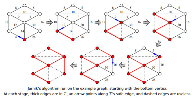
To implement Jarník’s algorithm, we keep all the edges adjacent to $T$ in a priority queue. When we pull the minimum-weight edge out of the priority queue, we first check whether both of its endpoints are in $T$. If not, we add the edge to $T$ and then add the new neighboring edges to the priority queue. In other words, Jarník’s algorithm is another instance of the generic graph traversal algorithm we saw last time, using a priority queue as the “bag”! If we implement the algorithm this way, the algorithm runs in $O(E \log E) = O(E \log V)$ time (because $E = V^2$ at most).

Similar to Dijkstra’s algorithm, if we implement the priority queue with a Fibonacci heap, the total running time would be $O(E + V \log V)$.

10.4 Kruskal’s Algorithm

Kruskal: Scan all edges in increasing weight order; if an edge is safe, add it to F.

def Kruskal(G):
	sort E w.r.t w
	
	F = (V, Ef)
	Ef <- Φ  # 空集
	
	for i <- 1 to E
		if E[i] is not useless
			Ef <- Ef + E[i]
			
	return F

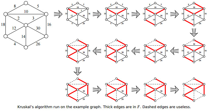
RT: $O(E \log E) = O(E \log V)$, dominated by the sorting.

11. Matroids (待续)

11.1 Definitions (待续)

A matroid $M$ is a finite collection of finite sets that satisfies three axioms:

• Non-emptiness: The empty set $\emptyset$ is in $M$. (Thus, $M$ is not itself empty.)
• Heredity: If a set $X$ is an element of $M$, then any subset of $X$ is also in $M$.
• Exchange: (a.k.a Augmentation) If $X$ and $Y$ are two sets in $M$ where $\lvert X \rvert > \lvert Y \rvert$, then there $\exists$ an element $x \in X \setminus Y$ such that $Y \cup \lbrace x \rbrace$ is in $M$.

• The sets in $M$ are typically called independent sets.
  • Therefore, the three axioms can also be stated as:
    • Non-emptiness: The empty set $\emptyset$ is independent.
    • Heredity: If a set $X$ is independent, then any subset of $X$ is also independent.
    • Exchange (a.k.a Augmentation): If $X$ and $Y$ are two independent sets where $\lvert X \rvert > \lvert Y \rvert$, then there $\exists$ an element $x \in X \setminus Y$ such that $Y \cup \lbrace x \rbrace$ is also independent.
• The union of all sets in $M$ is called the ground set.
  • In set theory, a collection, $F$, of subsets of a given set $S$ is called a family of subsets of $S$.
  • Therefore, a matroid is a family of subsets of its ground set.

• A maximal independent set is called a basis.
  • “Maximal” means it is not a proper subset of any other independent set. E.g.
    • Ground set $U = \lbrace 1,2,3 \rbrace$
    • $M = \lbrace \text{subsets of } U \text{ of size at most 2} \rbrace = \lbrace \emptyset, \lbrace 1 \rbrace, \lbrace 2 \rbrace, \lbrace 3 \rbrace, \lbrace 1,2 \rbrace, \lbrace 1,3 \rbrace, \lbrace 2,3 \rbrace \rbrace$
    • $\lbrace 1,2 \rbrace$, $\lbrace 1,3 \rbrace$ and $\lbrace 2,3 \rbrace$ are all bases.
  • The exchange property implies that every basis of a matroid has the same cardinality (i.e. size).
  • The rank of a matroid is the size of its bases.
• A subset of the ground set that is not in $M$ is a dependent set.
  • E.g. ground set $U = \lbrace 1,2,3 \rbrace$ itself is a dependent set above.
• A dependent set is called a circuit if any of its proper subset is independent.
  • E.g. ground set $U = \lbrace 1,2,3 \rbrace$ itself is a circuit above.

Here are several other examples of matroids; some of these we will see again later.

• Linear matroid: Let $A$ be any $n \times m$ matrix. A subset $I \subseteq \lbrace 1, 2, \dots, n \rbrace$ is independent if and only if the corresponding subset of columns of $A$ is linearly independent.
• Uniform matroid $U_{k,n}$: A subset $X \subseteq \lbrace 1, 2, \dots, n \rbrace$ is independent if and only if $\lvert X \rvert \leq k$. Any subset of $\lbrace 1, 2, \dots, n \rbrace$ of size $k$ is a basis; any subset of size $k + 1$ is a circuit.
• Matching matroid: Let $G = (V, E)$ be an arbitrary undirected graph. A subset $I \subseteq V$ is independent if there is a matching in $G$ that covers $I$.

TODO: Lecture note 和笔记本上还有些例子待补充。

11.2 Matroid Optimization Problem (待续)

Now suppose each element of the ground set of a matroid $M$ is given an arbitrary non-negative weight, i.e. $w: U \rightarrow \mathbb{R}^{+}$. The matroid optimization problem is to compute a basis with maximum total weight. For example, if $M$ is the cycle matroid for a graph $G$, the matroid optimization problem asks us to find the maximum spanning tree of $G$.

There goes a greedy alg:

# Given ground set U and matroid I
def GreedyMatroidOPT(U, I, w):
	B = Φ  # 空集
	
	# O(n log n)
	sort U w.r.t w in decreasing order
	
	# O(n)
	for each u ∈ U:
		# F(n)
		if B + {u} ∈ I:  # i.e. B + {u} is independent
			B = B + {u}
			
	return B

有没有觉得很像 Kruskal’s Algorithm？

RT: $O(n \log n) + n F(n)$. $F(n)$ 应该是 depends on 具体的应用。

TODO: 补充 proof

12. Matching (待续)

12.1 The Maximum Matching Problem

Let $G = (V, E)$ be an undirected graph. A set $M \subseteq E$ is a matching if no pair of edges in $M$ have a common vertex.

A vertex $v$ is matched if it is contained in an edge of $M$, and unmatched (or free) otherwise.

In the maximum matching problem we are asked to find a matching $M$ of maximum size.

12.2 Alternating and Augmenting Paths (待续)

Let $G = (V, E)$ be a graph and let $M$ be a matching in $G$. A path $P$ is said to be an alternating path with respect to $M$ if and only if among every two consecutive edges along the path, exactly one belongs to $M$. 我们也可以简称 $P$ is $M$-alternating.

E.g.

\[\begin{align} \in M & \notin M \in M \newline \text{===} & \text{--------} \text{===} \end{align}\]

If $A$ and $B$ are sets, let $A \oplus B = (A − B) \cup (B − A)$ be their symmetric difference. 其实就是异或（XOR）。

An augmenting path $P$ with respect to a matching $M$ is an alternating path that starts and ends in unmatched vertices, i.e. $P$’s endpoints are distinct free vertices. 我们也可以简称 $P$ is $M$-augmenting.

Lemma 2.3 If $M$ is a matching and $P$ is an alternating path with respect to $M$, where each endpoint of $P$ is either unmatched by $M$ or not, then $M \oplus P$ is also a matching.

这里你要把 $P$ 看做 edge 的集合，因为 path 用到了所有的边，所以 $P = E$。而 matching 不可能用到所有的边，所以 $M \subset E$，也就是 $\lvert M \rvert < \lvert E \rvert$。所以 $M \oplus P = M \oplus E = E \setminus M$。

下面有三条 alternating paths，粗线条的是 matching：

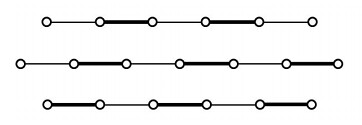
• CASE 1: If $P$ starts and ends in vertices unmatched by M (i.e. $P$ is $M$-augmenting) (e.g., the top path in figure), then $\lvert M \oplus P \rvert = \lvert M \rvert + 1$, i.e., $M \oplus P$ is a larger matching.
• CASE 2: If $P$ starts with an edge that does not belong to $M$ and ends with an edge of $M$ (e.g., the middle path in figure), then $\lvert M \oplus P \rvert = \lvert M \rvert$.
• CASE 3: If $P$ starts and ends with edges of $M$ (see the bottom path in figure 2), then $\lvert M \oplus P \rvert = \lvert M \rvert − 1$.

TODO: proof of CASE 1

Lemma 2.5 Let $G = (V, E)$ be an undirected graph and let $M_1$ and $M_2$ be matchings in $G$. Then, the subgraph $(V, M_1 \oplus M_2)$ is composed of isolated vertices, alternating paths and alternating cycles with respect to both $M_1$ and $M_2$.

Lemma 2.6 Let $G = (V, E)$ be an undirected graph and let $M$ and $M’$ be matchings in $G$ such that $\lvert M’ \rvert = \lvert M \rvert + k$, where $k \geq 1$. Then, there are at least $k$ vertex-disjoint augmenting paths in $G$ with respect to $M$. At least one of these augmenting paths is of length at most $\frac{n}{k} − 1$.

TODO: proof

Theorem 2.7 Let $G = (V, E)$ be an undirected graph and let $M$ be a matching in $G$. Then, $M$ is a maximum matching in $G$ if and only if there is no $M$-augmenting paths in G.

TODO: proof

Theorem 2.7 suggests the following simple algorithm for finding a maximum matching:

def MaxMatching(G):
	M = Φ  # 空集
	
	while exists an M-aug path P:
		M = M ⴲ P
			
	return M

• The while loop would take $\frac{V}{2}$ iteration.
• For bipartite graphs, AltBFS alg takes $O(E)$ time to find an $M$-aug path.

TODO: bipartite graphs & AltBFS alg

13. Testing Polynomial Identity (待续)

13.1 The Schwartz-Zippel Algorithm (待续)

检测两个 polynomial $Q$ 和 $R$ 是否相等，等价于检测是否有 polynomial $P = Q - R \equiv 0$ (i.e. 是否恒为 $0$).

首先来看 polynomial degree 的概念：

The degree of a polynomial is the highest degree of its terms when the polynomial is expressed in its canonical form consisting of a linear combination of monomials. The degree of a term is the sum of the exponents (指数) of the variables that appear in it.

比如 $x_1^2 x_2 + x_3 x_4 x_5^{10} + x_2^{11} x_3^{12}$，它有三个 terms：

• term $x_1^2 x_2$ 的 degree 是 $2 + 1 = 3$
• term $x_3 x_4 x_5^{10}$ 的 degree 是 $1 + 1 + 10 = 12$
• term $x_2^{11} x_3^{12}$ 的 degree 是 $11 + 12 = 23$
• 所以 polynomial 的 degree 等于 $\max \lbrace 3,12,23 \rbrace = 23$

The idea of the algorithm is very simple: assign values $r_1, \dots, r_n$ chosen independently and uniformly at random from a finite set $S$ to $x_1, \dots, x_n$. Test if $P(r_1, \dots, r_n) = 0$.

Claim 2.1 If $P \not\equiv 0$, then $Pr[P(r_1, \dots, r_n) = 0] \leq \frac{d}{\lvert S \rvert}$ where $d$ is the degree of $P$.

假设我们有 $\lvert S \rvert = 10d$，那么 $Pr[P(r_1, \dots, r_n) = 0] \leq \frac{1}{10}$。我跑它个 $n$ 次，它全为 0 的概率应该 $\leq (\frac{1}{10})^n$.

TODO: 补充证明

Digress: Permutation / Matrix Determinant (行列式)

onto function: A function $f: A \rightarrow B$ is called onto if $\forall b \in B$, $\exists a \in A$ such that $f(a) = b$, i.e. all elements in $B$ are used. Such functions are also referred to as surjective (满射).

one-to-one function: A function $f: A \rightarrow B$ is called one-to-one if whenever $f(a) = f(b)$ then $a = b$. No element of $B$ is the image of more than one element in $A$. Such functions are also referred to as injective (单射).

bijection: A functions that is both one-to-one and onto. Such functions are also referred to as bijective (双射).

A permutation of a set $X$ is a bijection $\pi: X \rightarrow X$. E.g. $\lbrace 1,2,3 \rbrace \rightarrow \lbrace 3,1,2 \rbrace$

• $\pi(1) = 3$
• $\pi(2) = 1$
• $\pi(3) = 2$

$\lbrace 1,2,3 \rbrace \rightarrow \lbrace 3,1,2 \rbrace$ 至少需要 2 swaps。 一次 swap 只能交换两个 elements。假设一个 permutation 变化至少需要 $k$ swaps，那么 sign of permutation $\operatorname{sign}(\pi) = (-1)^k$.

TODO: Prove that $\oepratorname{sign}$ is well defined, i.e. 对同一个 $\pi$，这个定义不可能产生不同的 $\operatorname{sign}(\pi)$。

Given an $n \times n$ matrix $A = [a_{i,j}]$, $Det(A) = \sum_{\pi}{\operatorname{sign}(\pi) \cdot a_{1,\pi(1)} \cdot a_{2,\pi(2)} \dots \cdot a_{n,\pi(n)}}$.

E.g. $n = 2$, $Det(A) = 1 \cdot a_{11} \cdot a_{22} + (-1) \cdot a_{12} \cdot a_{21}$.

• $\pi_1: \lbrace 1,2 \rbrace \rightarrow \lbrace 1,2 \rbrace $; $\operatorname{sign}(\pi_1) = 1$
• $\pi_2: \lbrace 1,2 \rbrace \rightarrow \lbrace 2,1 \rbrace $; $\operatorname{sign}(\pi_2) = -1$

13.2 Application to Bipartite Matching

Although bipartite matching is easy to solve in deterministic polynomial time using flow techniques, it remains an important open question whether there exists an efficient parallel deterministic algorithm for this problem.

Bipartite matching is the following problem: Given a bipartite graph $G = (V_1, V_2, E)$, where $\lvert V_1 \rvert = \lvert V_2 \rvert = n$, and all edges connect vertices in $V_1$ to vertices in $V_2$, does $G$ contain a perfect matching, that is, a subset of exactly n edges such that each vertex is contained in exactly one edge?

Definition 2.2 (Tutte matrix) The Tutte matrix $A_G$ corresponding to the graph $G$ is an $n \times n$ matrix $[a_{ij}]$ such that $a_{ij}$ is a variable $x_{ij}$ if $(i,j) \in E$, and $0$ otherwise.

Claim 2.3 $G$ contains a perfect matching if and only if $Det(A_G) \not\equiv 0$.

而且这个 perfect matching 可以被 $Det(A_G)$ 确定，比如：

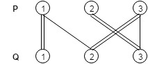
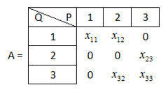
$Det(A) = - x_{11} \cdot x_{23} \cdot x_{32}$. 根据 $x_{ij}$ 的下标，我们可以看出 $\lbrace (p_1, q_1), (p_2, q_3), (p_3, q_2) \rbrace$ 是一个 perfect matching。

14. Eulerian Graph

Eulerian path: a path, $e_1 e_2 \cdots e_E$, which contains each edge exactly once.

Eulerian cycle: a closed Eulerian path.

Eulerian Graph: $G$ is Eulerian if it has an Eulerian cycle.

Thm: $G$ is Eulerian $\Leftarrow$ $G$ is connected and the degrees of all vertices are even.

Proof: Suppose every degree is even. We will show that there is an Euler cycle by induction on the number of edges in the graph.

The base case is for a graph $G$ with two vertices with two edges between them. This graph is obviously Eulerian.

Now suppose we have a graph $G$ on $m > 2$ edges. We start at an arbitrary vertex $v$ and follow edges, arbitrarily selecting one after another until we return to $v$. Call this path $W$. We know that we will return to $v$ eventually because every time we encounter a vertex other than $v$ we are listing one edge adjacent to it. There are an even number of edges adjacent to every vertex, so there will always be a suitable unused edge to list next. So this process will always lead us back to $v$.

Let $E_W$ be the edges of $W$. The graph $G − E_W$ has components $C_1, C_2, \cdots, C_k$. These each satisfy the induction hypothesis: connected, less than $m$ edges, and every degree is even. We know that every degree is even in $G − E_W$, because when we removed $W$, we removed an even number of edges from those vertices listed in the cycle. By induction, each component has an Eulerian cycle, call them $E_1, E_2, \cdots, E_k$.

Since $G$ is connected, there is a vertex $a_i$ in each component $C_i$ on both $W$ and $E_i$. Without loss of generality, assume that as we follow $W$, the vertices $a_1, a_2, \cdots, a_k$ are encountered in that order.

We describe an Euler cycle in $G$ like this:

• Starting at $v$;
• Follow $W$ until reaching $a_1$, follow the entire $E_1$ ending back at $a_1$;
  • follow $W$ until reaching $a_2$, follow the entire $E_2$, ending back at $a_2$ and so on;
    • follow $W$ until reaching $a_k$, and follow the entire $E_k$, ending back at $a_k$.
• Finish off $W$, ending at $v$.

Thm: Odd-order complete graph is Eulerian.

• Let $K_n$ be the complete graph of $n$ vertices.
• Then $K_n$ is Eulerian if and only if $n$ is odd.
• If $n$ is even, then $K_n$ is traversable iff $n=2$.
  • If a graph is not traversable, it cannot be Eulerian.

15. Hamiltonian Path

Hamiltonian path: a simple path that contains all vertices.

Hamiltonian cycle: a simple cycle that contains all vertices.

• “simple” means “containing each edge exactly once”.

Hamiltonian path/cycle problems are of determining whether a Hamiltonian path/cycle exists in a given graph (whether directed or undirected). Both problems are NP-complete.

There is a simple relation between the problems of finding a Hamiltonian path and a Hamiltonian cycle.

• In one direction, the Hamiltonian path problem for graph $G$ is equivalent to the Hamiltonian cycle problem in a graph $H$ obtained from $G$ by adding a new vertex and connecting it to all vertices of $G$. Thus, finding a Hamiltonian path cannot be significantly slower (in the worst case, as a function of the number of vertices) than finding a Hamiltonian cycle.
• In the other direction, the Hamiltonian cycle problem for a graph $G$ is equivalent to the Hamiltonian path problem in the graph $H$ obtained by copying one vertex $v$ of $G$, $v’$, that is, letting $v’$ have the same neighbourhood as $v$, and by adding two dummy vertices of degree one, and connecting them with $v$ and $v’$, respectively.
  • The Hamiltonian cycle problem is also a special case of TSP (travelling salesman problem).

A brute-force alg: try every permutation of vertices (that’s $O(V!)$), see if there is any Hamiltonian cycle.

An $O(V^2 2^V)$ DP alg: BellmanHeldKarp. (已知 $V^2 2^V \ll V!$)

$V = \lbrace v_1, \dots, v_n \rbrace, n = \vert V \vert, S \subseteq V$

\[\begin{equation} H(v_i,S) = \begin{cases} True & \exists \text{ a Hamiltonia path from } v_1 \text{ to } v_i \text{ with all vertices in } S \newline False & \text{otherwise} \end{cases} \end{equation}\]

$H(v_n,V)$ is our aim.

$H(v_i,S) = \exists j \text{ s.t. } H(v_j,S \setminus \lbrace v_i \rbrace) \text { & } (v_i, v_j) \in E$

Base Case: $H(v_1, \lbrace v_1 \rbrace) = True$

$\exists$ a Hamiltonia cycle if $\exists j \text{ s.t. } H(v_j,V) = True \text { & } (v_1, v_j) \in E$

DP table: (# of $v_i$) $\times$ $\lvert S \rvert$ = $V \times 2^V$

RT: time to fill a cell $\times$ DP table size = $V \times V \times 2^V = V^2 2^V$’