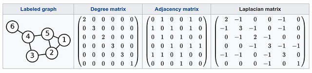
Laplacian Matrix

1. DefinitionPermalink

Quote from Wikipedia: Laplacian matrix:

Given a simple graph $G$ with $n$ vertices, its Laplacian matrix $L_{n\times n}$ is defined as:

$$L=D-A,$$

where $D$ is the degree matrix and $A$ is the adjacency matrix of the graph. Since $G$ is a simple graph, $A$ only contains $1$s or $0$s and its diagonal elements are all $0$s.

In the case of directed graphs, either the indegree or outdegree might be used, depending on the application.

The elements of $L$ are given by:

E.g., here is a simple example of undirected graph and its Laplacian matrix.

至于 Symmetric normalized Laplacian 和 Random-walk normalized Laplacian 请看 Wikipedia

2. Why is it called “Laplacian”?Permalink

这里其实是一个 analog：

• Graph $G(E,V)\leftrightarrow$ Function $f(x)$
• $G$ 的 Laplacian Matrix $\leftrightarrow$ $f$ 的 ${\mathrm{\nabla }}^2$ operator

2.1 Prerequisite: Incidence MatrixPermalink

A $|E|\times |V|$ matrix for graph $G(E,V)$.

Oriented incidence matrices are for directed graphs:

while unoriented incidence matrices for undirected graphs:

2.2 An ExamplePermalink

Muni Sreenivas Pydi’s answer to “What’s the intuition behind a Laplacian matrix?” on Quora is a fantastic one. Well appreciated!

首先把 $G=(V,E)$ 类比成一个函数 $f(v)=\mathrm{degree}(v)$。然后我们自己定义 gradient of graph $\mathrm{\nabla }f{\mid }_{e=(u,v)}=f(u)-f(v)$，即沿着 $e$ 的方向上的 degree 的变化。

注意这里有几个问题：

• 这个答案本质上是把 $G$ 当做 undirected graph 处理：
  • $f(v)$ 的定义用的是 degree 而不是 in-degree 或者 out-degree
  • 后面 $G$ 的 degree matrix 和 adjacency matrix 也是按 undirected graph 的算法算的
• 但是他的 $E$ 是有方向的。这完全是人为的规定，因为如果不定义 $E$ 的方向，讨论起来就很麻烦，而且 $E$ 的方向其实不重要：假设 $e=(u,v)，\mathrm{\nabla }f{\mid }_e=2$，那么如果我们定义 $e=(v,u)$，那么很明显这时的 $\mathrm{\nabla }f{\mid }_e=-2$。方向仅仅会改变最终结果的正负号而已，不影响你理解整个的思想。

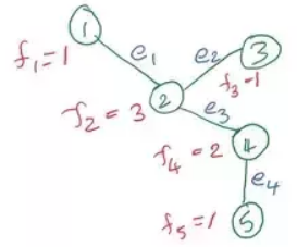
$E$ 的方向是：

• $e_1=(1,2)$
• $e_2=(2,3)$
• $e_3=(2,4)$
• $e_4=(4,5)$

定义：

Incidence matrix:

所以有：

类似地，$\mathrm{div}(\mathrm{grad}f)$ 可以理解为在每个 vertex 上 degree 的增量的变化，比如：

• 你可以想象成 degree 大多从 $v_2$ 流出
• $v_1$ 和 $v_3$ 接收流入的 degree（来自 $v_2$），且没有 degree 流出
• $v_3,v_4$ 没有直接相连，不存在 degree 的流动，所以 divergence 为 0

我们单独看一下 $K^{T}K$:

而 $G$ 的 Laplacian matrix 是:

Suprisingly:

所以，我们称 $L$ 为 Laplacian matrix 是因为它真的可以和 Laplace operator 联系起来！

另外注意 $L$ 的对角线刚好为 matrix $f$

3. 扩展Permalink

3.1 可以定义不同的 $f$Permalink

$K^{T}Kf$ 表示的就是 “extent to which values of $f$ change from one vertex to another connected vertex in $G$”。更直观一点描述的话：

• 考虑 $K^{T}Kf$ vector 元素全部为 0 的情况。这说明在 $G$ 上沿着 vertex 一步一步前进时，$f$ 的值是绝对 smooth 的，没有变化。
• 如果 $K^{T}Kf$ vector 元素 highly postive 或者 highly nagative，说明 $f$ 的起伏很大。
• 所以 $K^{T}Kf$ 描述的是 $f$ 在 $G$ 上的 smoothness

至于 $f$ 具体是什么，你可以根据你自己的 application 去定义。

3.2 可以引入 weight $w$Permalink

Quote from The Laplacian by Daniel A. Spielman, Yale:

Adjacency matrix of a weighted graph $G=(E,V)$:

Degree matrix is a diagonal matrix such that:

Laplacian matrix of such a weighted graph $G$ is $L^{(w)}=D-A$. Hence,

(Note: This is the Dirichlet energy of a graph function $f$.)

Prove: Here we introduce a simpler way to define Laplacian matrix.

If we only consider 2 vertices $u,v$ and define

Then we have $(f(u)-f(v){)}^2=[\begin{array}{cc}f(u)& f(v)\end{array}]L_{u,v}[\begin{array}{c}f(u)\\ f(v)\end{array}]$

Note that if the conventional Laplacian matrix of $G$, when weights are not taken into account, is $L$, we’ll have

It’s a hint that $L$ can be represented by $L_{u,v}$ and actually we have:

where $\mathrm{expand}$ casts the $2\times 2$ matrix $L_{u,v}$ into a $|V|\times |V|$ one whose only non-zero entries are in the intersections of rows and columns $u$ and $v$.

E.g. consider a simple graph $(a)—(b)—(c)$

Therefore,

Similarly, we can define:

Thus, $w(u,v)\cdot (f(u)-f(v){)}^2=[\begin{array}{cc}f(u)& f(v)\end{array}]L_{u,v}^{(w)}[\begin{array}{c}f(u)\\ f(v)\end{array}]$.

Therefore, we can further define,

E.g. consider a simple weighted graph $(a)\stackrel{3}{—}(b)\stackrel{2}{—}(c)$

At the same time,

3.3 可以转化成一个优化问题：求最优的 $f^{\prime }=\underset{f}{\arg min}{f}^{T}Lf$Permalink

If you dig a little deeper, you may notice that the functions that minimize the expression $f^{T}Lf$ are the eigenvectors the the Laplacian! For unit norm functions, this expression is just the Rayleigh quotient of the Laplacian matrix. And by Min-max theorem, we have that the solutions to this minimization are just the eigenvectors!

Basically, the first eigenvector of the graph Laplacian is the smoothest function you can find on the graph. In case of a connected graph, it is the constant function. The second eigenvector is the next smoothest function of all graph functions that are orthogonal to the first one and so on. You can even think of the first eigenvector of the Laplacian as the DC component of the graph signal. The next eigenvectors are just the higher frequency modes of the signal. In fact, the eigenvectors of the Laplacian form an orthonormal Fourier basis for the space of graph functions! This tangent leads us to an exciting research area called graph signal processing.