Computational Complexity Review

March 30, 2016 73 minute read

1. Turing Machines @ Automata by Jeff Ullman

1.1 Introduction

Questions:

How to show that certain tasks are impossible, or in some cases, possible but intractable?
- Intractable means solvable but only by very slow algorithms
What can be solved by computer algorithms?

Turing machine (TM):

In some sense an ultimate automaton.
A formal computing model that can compute anything we can do with computer or with any other realistic model that we might think of as computing.
TMs define the class of recursively enumerable languages which thus the largest class of languages about which we can compute anything.
- There is another smaller class called recursive languages that can be thought of as modeling algorithms–computer programs that answer a particular question and then finish.

1.2 Data

Data types:

int, float, string, etc.
But at another level, there is only one type $\Rightarrow$ string of bit.
- It is more convenient to think of binary strings as integers.
Programs are also strings and thus strings of bits.
- The fact that programs and data are at heart the same thing is what let us build a powerful theory about what is not computable.

“The $i^{th}$ data”:

Integers $\Rightarrow 1, 2, 3, \dots$
“Data” can also be mapped to $1, 2, 3, \dots$ (with some tricks from coding or cryptography)
- Then it makes sense to talk about “the $i^{th}$ data”
E.g. “the $i^{th}$ string”:
- Text strings (ASCII or Unicode) $\Rightarrow$ Binary strings $\overset{\textrm{encode}}{\Rightarrow}$ Integers
  - A small glitch: If you think simply of binary integers, then
    - $101$ $\Rightarrow$ “the $5^{th}$ string”
    - $0101$ $\Rightarrow$ “the $5^{th}$ string”
    - $00101$ $\Rightarrow$ “the $5^{th}$ string”
- This can be fixed by prepending a $1$ to the string before converting to an integer. Thus,
  - $101$ $\Rightarrow$ “the $13^{th}$ string” ($\color{red}{1}101 = 13$)
  - $0101$ $\Rightarrow$ “the $21^{st}$ string” ($\color{red}{1}0101 = 21$)
  - $00101$ $\Rightarrow$ “the $37^{th}$ string” ($\color{red}{1}00101 = 37$)
E.g. “the $i^{th}$ proof”:
- A formal proof is a sequence of logical expressions.
  - We can encode mathematical expressions of any kind in Unicode.
  - Convert expression to a binary string and then an integer.
- Problems:
  - A proof is a sequence of expressions, so we need a way to separate them.
  - Also, we need to indicate which expressions are given and which follow from previous expressions.
- Quick-and-dirty way to introduce special symbols into binary strings:
  1. Given a binary string, precede each bit by 0. E.g.:
    - $101$ becomes $010001$.
  2. Use strings of two or more $1$’s as the special symbols. E.g.:
    - Let $111$ mean “start of expression”
    - Let $11$ mean “end of expression”
- E.g. $\color{blue}{111}\color{red}{0}\underline{1}\color{red}{0}\underline{0}\color{red}{0}\underline{1}\color{blue}{11}\color{cyan}{111}\color{red}{0}\underline{0}\color{red}{0}\underline{0}\color{red}{0}\underline{1}\color{red}{0}\underline{1}\color{cyan}{11} = \underline{101},\underline{0011}$

1.3 Orders of infinity

There aren’t more “data” than there are integers.
While the number is infinite, you may aware that there are different orders of infinity, and the integers is of the smallest one.
- E.g. there are more real numbers than there are integers, so there are more real numbers than there are “programs” (think of programs as data).
  - This immediately tells you that some real numbers cannot be computed by programs.

1.3.1 Finite sets

A finite set has a particular integer that is the count of the number of members–the cardinality.
- E.g. $\operatorname{card}(\lbrace a, b, c \rbrace) = 3$
It is impossible to find a 1-to-1 mapping between a finite set and a proper subset of itself.

1.3.2 Infinite Sets

Formally, an infinite set is a set for which there is a 1-to-1 mapping between itself and a proper subset of itself.
- E.g. the positive integers $\lbrace 1, 2, 3, \dots \rbrace$ is an infinite set.
  - There is a 1-to-1 mapping $1 \mapsto 2, 2 \mapsto 4, 3 \mapsto 6, \dots$ between this set and a proper subset (the set of even integers).

1.3.3 Countable Sets

A countable set is a set with a 1-to-1 mapping with the positive integers.
- $\Rightarrow$ Hence, all countable sets are infinite.
E.g. set of all integers:
- $0 \mapsto 1$
- $-x \mapsto 2x$
- $+x \mapsto 2x+1$
- Thus, order is $0, -1, 1, -2, 2, -3, 3,…$, i.e.
  - $1^{st}$ integer is $0$
  - $2^{nd}$ integer is $-1$
  - etc.
E.g. set of binary strings, set of Java programs.
E.g. pairs of integers
- Order the pairs of positive integers first by sum, then by first component: $[1,1], [2,1], [1,2], [3,1], [2,2], [1,3], [4,1], [3,2], \dots, [1,4], [5,1], \dots$
- $[i,j] \mapsto f(i,j) = \frac{(i+j)(i+j-1)}{2} - i + 1 = \frac{(i+j-1)(i+j-2)}{2} + j$

1.3.4 Enumerations

An enumeration of a set is a 1-to-1 mapping between the set and the positive integers.
Thus, we have seen enumerations for strings, programs, proofs, and pairs of integers.

1.3.5 Set of all languages over some fixed alphabet

Question: Are the languages over $\lbrace 0,1 \rbrace$ countable?

Answer: No. Proof by Diagonalization (a table of $m$ strings $\times$ $n$ languages):

Suppose we could enumerate all languages over $\lbrace 0,1 \rbrace$ and talk about “the $i^{th}$ language.”

Consider the language:

\[L = \lbrace w \vert w \, \text{is the} \, i^{th} \, \text{binary string and} \, w \, \text{is not in the} \, i^{th} \, \text{language} \, \rbrace\]

Clearly, $L$ is a language over $\lbrace 0,1 \rbrace$.

Thus, $L$ is the $j^{th}$ language for some particular $j$.

Let $x$ be the $j^{th}$ string. Is $x$ in $L$?

If so, $x$ is not in $L$ by definition of $L$.
If not, then $x$ is in $L$ by definition of $L$.

We have a contradiction: $x$ is neither in $L$ nor not in $L$, so our sole assumption (that there was an enumeration of the languages) is wrong. $\blacksquare$

This is really bad; there are more languages than programs:

The set of all programs are countable
The set of all languages are not countable

1.4 Turing-Machine

Turing-Machine Theory:

One important purpose of the theory of Turing machines is to prove that certain specific languages have no membership algorithm.
The first step is to prove certain languages about Turing machines themselves have no membership algorithm.
Reductions are used to prove more common questions undecidable.

Picture of a Turing Machine:

Finite number of states.
Infinite tape with cells containing tape symbols chosen from a finite alphabet.
- Tape head: always points to one of the tape cells.
Action: based on the state and the tape symbol under the head, a TM can
- change state
- overwrite the current symbol
- move the head one cell left or right

Why Turing Machines? Why not represent computation by C programs or something like that?

You can develop a theory about programs without using Turing machines, but it is easier to prove things about TM’s, because they are so simple.
And yet they are as powerful as any computer.
- In fact, TMs are more powerful than any computer, since they have infinite memory
  - Yes, we could always buy more storage for a computer.
  - But the universe is finite so where are you going to get the atoms from which to build all of those discs?
  - However, once you accept that the universe is finite, the limitation doesn’t seem to be effecting what we can compute in practice.
  - So we are not going to argue that a computer is weaker than a Turing machine in a meaningful way.

1.4.1 Turing-Machine Formalism

A TM is typically described by:

A finite set of states, $Q$
An input alphabet, $\Sigma$
- symbol 和 alphabet 的关系是 $\text{symbol} \in \text{alphabet}$
A tape alphabet, $\Gamma$
- $\Sigma \subseteq \Gamma$
A transition function, $\delta$
A start state, $q_0 \in Q$
A blank symbol, $B \in \Gamma \setminus \Sigma$
- All tape except for the input is blank initially.
- $B$ is never an input symbol.
A set of final states, $F \subseteq Q$

Conventions:

$a, b, \dots$ are input symbols.
$\dots, X, Y, Z$ are tape symbols.
$\dots, w, x, y, z$ are strings of input symbols.
$\alpha, \beta, \dots$ are strings of tape symbols.

Transition Function $\delta(q, Z) = (p, Y, D)$:

Arguments:
1. Current state $q \in Q$
2. Current tape symbol $Z \in \Gamma$
Return value (when $\delta(q, Z)$ in not undefined):
- $p$ is a state
- $Y$ is the new tape symbol (to replace the current symbol on the tape head)
- $D$ is a direction, $L$ or $R$

TM Example:

Description:
- This TM scans its input (all binary bits) left to right, looking for a 1.
- If it finds 1, it changes it to a 0, goes to final state $f$, and halts.
- If it reaches a blank, it changes it to a 1 and moves left.
Formalism:
- States $Q = \lbrace q \, \text{(start)}, f \, \text{(final)} \rbrace$.
- Input symbols $\Sigma = \lbrace 0, 1 \rbrace$.
- Tape symbols $\Gamma = \lbrace 0, 1, B \rbrace$.
- $\delta(q, 0) = (q, 0, R)$.
- $\delta(q, 1) = (f, 0, R)$.
- $\delta(q, B) = (q, 1, L)$.
Example tape: $BB00BB$; starts from the first 0
- $BB\color{red}{0}0BB$, $\delta(q, 0) = (q, 0, R)$, move right
- $BB0\color{red}{0}BB$, $\delta(q, 0) = (q, 0, R)$, move right
- $BB00\color{red}{B}B$, $\delta(q, B) = (q, 1, L)$, move left
- $BB0\color{red}{0}1B$, $\delta(q, 0) = (q, 0, R)$, move right
- $BB00\color{red}{1}B$, $\delta(q, 1) = (f, 0, R)$, move right
- $BB000\color{red}{B}$, undefined, halt.

Instantaneous Descriptions of a Turing Machine:

Initially, a TM has a tape consisting of a string of input symbols surrounded by an infinity of blanks in both directions.
The TM is in the start state, and the head is at the leftmost input symbol.
TM ID’s: (我觉得更合适的名字应该叫 TM State ID)
- An ID is a string $\alpha q \beta$, where
  - $\alpha =$ string from the leftmost nonblank to tape head (exclusive)
  - $\beta =$ string from the tape head (inclusive) to the rightmost nonblanks.
    - I.e. the symbol to the right of $q$ is the one being scanned.
  - If an ID is in the form of $\alpha q$, it is scanning a $B$.
- As for PDA’s (Pushdown automaton) we may use symbols
  - $ID_i \vdash ID_j$ to represent “$ID_i$ becomes $ID_j$ in one move” and
  - $ID_i \vdash^{\star} ID_j$ to represent “$ID_i$ becomes $ID_j$ in zero or more moves,”。
- Example: The moves of the previous TM are $q00 \vdash 0q0 \vdash 00q \vdash 0q01 \vdash 00q1 \vdash 000f$
Formal Definition of Moves:
1. If $\delta(q, Z) = (p, Y, R)$, then
  - $\alpha qZ \beta \vdash \alpha Yp \beta$
  - If $Z$ is the blank $B$, then $\alpha q \vdash \alpha Yp$
2. If $\delta(q, Z) = (p, Y, L)$, then
  - For any $X$, $\alpha XqZ \beta \vdash \alpha pXY \beta$
  - In addition, $qZ \beta \vdash pBY \beta$

1.4.2 Languages of a TM

There are actually two ways to define the language of a TM:

A TM defines a language by final state.
- $L(M) = \lbrace w \vert q_0 w \vdash^{\star} I, \, \text{where I is an ID with a final state} \rbrace$
Or, a TM can accept a language by halting.
- $H(M) = \lbrace w \vert q_0 w \vdash^{\star} I, \, \text{and there is no move possible from ID} \, I \rbrace$

Equivalence of Accepting and Halting:

If $L = L(M)$, then there is a TM $M’$ such that $L = H(M’)$.
If $L = H(M)$, then there is a TM $M”$ such that $L = L(M”)$.

Proof:

Final State => Halting:

Modify $M$ to become $M’$ as follows:
1. For each final state of $M$, remove any moves, so $M’$ halts in that state.
2. Avoid having $M’$ accidentally halt.
  - Introduce a new state $s$, which runs to the right forever; that is $\delta(s, X) = (s, X, R)$ for all symbols $X$.
  - If $q$ is not a final state, and $\delta(q, X)$ is undefined, let $\delta(q, X) = (s, X, R)$.

Halting => Final State:

Modify $M$ to become $M”$ as follows:
1. Introduce a new state $f$, the only final state of $M”$.
2. $f$ has no moves.
3. If $\delta(q, X)$ is undefined for any state $q$ and symbol $X$, define it by $\delta(q, X) = (f, X, R)$. $\blacksquare$

Recursively Enumerable Languages:

We now see that the classes of languages defined by TM’s using final state and halting are the same.
This class of languages (that can be defined in both those ways) is called the recursively enumerable languages.
- Why this name? The term actually predates the Turing machine and refers to another notion of computation of functions.

Recursive Languages:

A proper subset of Recursively Enumerable Languages.
An algorithm formally is a TM accepting (a language) by final state that halts on any input regardless of whether that input is accepted or not.
- 注意这里的逻辑，algorithm 是 TM 而不是 language.
If $L = L(M)$ for some TM $M$ that is an algorithm, we say $L$ is a recursive language.
- In other words, the language that is accepted by final state by some algorithm is a recursive language.
- Why this name? Again, don’t ask; it is a term with a history.
Example: Every CFL (Context-free language) is a recursive language.
- By the CYK algorithm.

2. Decidability @ Automata by Jeff Ullman

Central Ideas:

TMs can be enumerated, so we can talk about “the $i^{th}$ TM”.
- Thus possible to diagonalize over TMs, showing a language that cannot be the language of any TM.
Establish the principle that a problem is really a language.
- Therefore some specific problems do not have TMs.

Binary-Strings from TM’s:

We shall restrict ourselves to TM’s with input alphabet $\lbrace 0, 1 \rbrace$.
Assign positive integers to the three classes of elements involved in moves:
1. States: $q_1$ (start state), $q_2$ (final state), $q_3$, etc.
2. Symbols: $X_1$ (0), $X_2$ (1), $X_3$ (blank), $X_4$, etc.
3. Directions: $D_1$ (L) and $D_2$ (R).
Suppose $\delta(q_i, X_j) = (q_k, X_l, D_m)$.
Represent this rule by string $0^i10^j10^k10^l10^m$. ($0^n$ 表示 $n$ 个连续的 $0$)
- Key point: since integers $i, j, \dots$ are all $> 0$, there cannot be two consecutive $1$’s in these strings.
Represent a TM by concatenating the codes for each of its moves, separated by $11$ as punctuation.
- That is: $\text{Code}_111\text{Code}_211\text{Code}_311\dots$
- Note: if bianry string $i$ cannot be parsed as a TM, assume the $i^{th}$ TM accepts nothing.

Diagonalization:

Table of Acceptance (denoted by $A$):
- TM $i=1,2,3,\dots$ $\times$ String $j=1,2,3,\dots$
- $A_{ij} = 0$ means the $i^{th}$ TM does not accept the $j^{th}$ string.
- $A_{ij} = 1$ otherwise.
Construct a 0/1 sequence $D=d_1 d_2 \dots$, where $d_i = \overline{A_{ii}}$
- $D$ cannot be a row in $A$.
- Question: Let’s suppose $w=10101010\dots$. What does it mean if $w$ appears in the $i^{th}$ row of the table $A$?
- Answer: It means the $i^{th}$ TM exactly accepts the $1^{st}, 3^{rd}, 5^{th}, \dots$ binary strings.
Let’s give a name to this language–the diagonalization language $L_d = \lbrace w \vert w \text{ is the } i^{th} \text{ string, and the } i^{th} \text{ TM does not accept } w \rbrace$.
We have shown that $L_d$ is not a recursively enumerable language; i.e., it has no TM.
- There are no more TMs than integers.
- $L_d$ exists but we cannot always tell whether a given binary string $w$ is in $L_d$.

Problems:

Informally, a “problem” is a yes/no (the output) question about an infinite set of possible instances (the input).
- Example: “Does graph G have a Hamilton cycle (cycle that touches each node exactly once)?
- Each undirected graph is an instance of the “Hamilton-cycle problem.”
Formally, a problem is a language.
- Each string encodes some instance.
- The string is in the language if and only if the answer to this instance of the problem is “yes.”
Example: A Problem About Turing Machines
- We can think of the language $L_d$ as a problem.
- 如果 table $A$ 的 string 是 TM 自身的 binary string 的话，这个 problem 就成了 “Does this TM not accept its own code?”

Decidable Problems:

A problem is decidable if there is an algorithm to answer it.
- Recall: An “algorithm,” formally, is a TM that halts on all inputs, accepted or not.
- Put another way, “decidable problem” = “recursive language.”
Otherwise, the problem is undecidable.

Bullseye Picture:

最中心的集合：Decidable problems = Recursive languages
外一圈：Recursively enumerable languages
- Languages accepted by TMs with no guarantee that they will halt on inputs they never accept
- Recursively enumerable languages $\supset$ Recursive languages
最外层：Not recursively enumerable languages，比如 $L_d$
- Languages that have no TM at all.
- Recursively enumerable languages 的补集

Examples: Real-world Undecidable Problems

Can a particular line of code in a program ever be executed?
Is a given context-free grammar ambiguous?
Do two given CFG’s generate the same language?

The Universal Language:

An example of a recursively enumerable, but not recursive language
We call it $L_u$, of a universal Turing machine, or call it Universal TM language.
UTM inputs include:
- a binary string representing some TM $M$, and
- a binary string $w$ for $M$
UTM accepts $\langle M,w \rangle$ if and only if $M$ accepts $w$.
E.g. JVM
- JVM takes a coded Java program and input for the program and executes the program on the input.

Designing the UTM:

Inputs are of the form: $\text{Code–for–}M \, 111 \, w$
- Note: A valid TM code never has $111$, so we can split $M$ from $w$.
- The UTM must accept its input if and only if $M$ is a valid TM code and $M$ accepts $w$.
UTM is a multi-tape machine:
- Tape 1 holds the input $\text{Code–for–}M \, 111 \, w$
  - Tape 1 is never changed, i.e. never overwritten.
- Tape 2 represents the current tape of $M$ during the simulation of $M$ with input $w$
- Tape 3 holds the state of $M$.
Step 1: The UTM checks that $M$ is a valid code for a TM.
- E.g., all moves have five components, no two moves have the same state/symbol as first two components.
- If $M$ is not valid, its language is empty, so the UTM immediately halts without accepting.
Step 2: Assuming the code for $M$ is valid, the UTM next examines $M$ to see how many of its own tape cells it needs to represent one symbol of $M$.
- How to do this: we discover the longest block of $0$s representing a tape symbol and add one cell to that for a marker (e.g. $\text{#}$) between symbols of $M$’s tape.
- Thus if say $X_7$ is the highest numbered symbol then we’ll use 8 squares to represent one symbol of $M$.
  - Symbol $X_i$ will be represented $i$ $0$s and $7-i$ blanks followed by a marker outside.
  - For example, here’s how we would represent $X_5$: $00000BB\text{#}$.
Step 3: Initialize Tape 2 to represent the tape of $M$ with input $w$, and initialize Tape 3 to hold the start state (always $q_1$ so it is represented by a single $0$).
Step 4: Simulate $M$.
- Look for a move on Tape 1 that matches the state on Tape 3 and the tape symbol under the head on Tape 2.
  - If we cannot find one then apparently $M$ halts without accepting $w$ so UTM does so as well.
- If found, change the symbol and move the head on Tape 2 and change the State on Tape 3.
- If $M$ accepts (i.e. halts), the UTM also accepts (i.e. halts).

Proof That $L_u$ is Recursively Enumerable (RE), but not Recursive:

We designed a TM for $L_u$, so it is surely RE.
Proof by contradiction:
- Suppose $L_u$ were recursive, which means we could design a UTM $U$ that always halted.
- Then we could also design an algorithm for $L_d$, as follows.
  - Given input $w$, we can decide if $w \in L_d$ by the following steps.
    1. Check that $w$ is a valid TM code.
      - If not, then $w$’s language is empty, so $w \in L_d$.
    2. If valid, use the hypothetical algorithm to decide whether $w \, 111 \, w$ is $\in L_u$.
    3. If so, then $w \notin L_d$; else $w \in L_d$.
- But we already know there is no algorithm for $L_d$.
- Thus, our assumption that there was an algorithm for $L_u$ is wrong.
- $L_u$ is RE, but not recursive.

$\blacksquare$

这个证明需要好好解读与总结：

什么是 language?
- TM $M$ 的 language $L_M = \lbrace \text{tape (不算两端的 blank 区域)} \vert \text{TM 能从这个 tape 的起始点一直运行到一个 final state, i.e. halt} \rbrace$
- Tape 的本质是什么？是 string 呀
- 我们说 TM $M$ accepts a language，那么同样也可以说 TM $M$ accepts a string，然后所有 $M$ accept 的 string 构成了 $M$ 的 language
什么是 algorithm?
- algorithm 是个 TM, which always halts on any input regardless of whether that input is accepted or not
  - always halts 是什么意思？你可以理解为 “always generate an output”
    - accept 输出 1
    - reject 输出 0
  - 明显，infinite loop 不可能是一个 algorithm
什么是 problem?
- problem is a language
TM accept a language => algorithm accepts a problem
- 但是我们一般不这么说，因为我们常用的说法是 algorithm solves a problem
- 反过来，a problem is solved by algorithm，也就相当于 “我们可以为 problem 这个 language 找到一个 always halt 的 TM，即找到一个 algorithm”
  - 能找到 algorithm 的 problem => Decidable Problem, i.e. Recursive language
  - 能找到 TM (但不保证是 algorithm) 的 problem => Recursively enumerable language
    - 能找到 TM，但确定不是 algorithm 的 problem => The Universal Language
  - 连 TM 都找不到的 problem => Not recursively enumerable language
$w$ 的两面性
- 如果 TM $M$ 的 binary string 是 $w$，那么
  1. $w$ 可以表示 TM $M$
  2. $w$ 可以表示一个 plain string
- 那么我们可以同时有 “$w$ accepts $w$” 和 “$w$ is accepted by $w$” 这两种逻辑
$L_d$ 的两种解读
- 首先它是个 language，然后 language 可以看做一个集合；然后 problem 也是 language，所以也把 $L_d$ 抽象成一个问题描述
- 貌似默认是把 Acceptance table $A$ 的 string 限定为 TM 的 binary string 的话（相当于是 $w \times w$ 这样的一张表），那么：
  - $L_d = \lbrace w \vert \text{TM } w \text{ does not accept string } w \rbrace$
    - 你理解为 string 的集合或者 TM 的集合都行，因为 $w$ 的两面性
    - 原来的定义是 $L_d = \lbrace w \vert w \text{ is the } i^{th} \text{ string, and the } i^{th} \text{ TM does not accept } w \rbrace$，请自行体会一下是不是可以这么理解
  - $L_d$ is a problem “Does this TM not accept its own code?”
If $w$ is not a valid TM code:
- 有点无赖地，我们把这样的 $w$ 看做一种特殊的 TM
- $w$’s language is empty
  - => $w$ accepts nothing
    - => $w$ cannot accept $w$
      - => $w \in L_d$
$L_u$ 没有 algorithm 意味着什么？
- 给定一个 $\langle M, w \rangle$，没有 algorithm 确定是否有 $M$ accepts $w$
- 还是回到 “$w$ accepts $w$” 这个逻辑上，然后我们可以把 $\langle w, w \rangle$ 写成 $w \, 111 \, w$，所以针对这个输入，没有 algorithm 可以确定是否有 $w$ accepts $w$

3. Extensions and properties of Turing machines @ Automata by Jeff Ullman

17.1 Programming Tricks

Programming Trick: Multiple Tracks

Enable us to leave markers on the tape so TM can find their way back to an important place.
If there are $k$ tracks => Treat each symbol as a vector of size $k$
- E.g. $k=3$. $\left( \begin{smallmatrix} 0 \newline 0 \newline 0 \end{smallmatrix} \right)$ represents symbol $0$; $\left( \begin{smallmatrix} B \newline B \newline B \end{smallmatrix} \right)$ represents blank; $\left( \begin{smallmatrix} X \newline Y \newline Z \end{smallmatrix} \right)$ represents symbol $[X,Y,Z]$

Programming Trick: Marking

$k-1$ tracks for data; 1 track for marks
Almost all tape cells hold blank in this mark track, but several hold special symbols (marks) that allow the TM to find particular places on the tape.
E.g. $\left( \begin{smallmatrix} B & X & B \newline W & Y & Z \end{smallmatrix} \right)$ represents an unmarked $W$, a marked $Y$ and an unmarked $Z$ ($X$ is a mark)

Programming Trick: Caching in the State

Treat state as a vector.
First component is the “control state,” i.e. the orginal state
Other components are used as a cache to hold values the TM needs to remember.

例子待续

17.2 Restrictions

Semi-infinite Tape: 待续

17.3 Extensions

Multitape TM:

To simulate a $k$-Tape TM, use $2 \times k$ tracks ($2 \times k$ tracks 仍然视为一个 tape；$k$-Tape 是要有 $k$ 个 head 的)
For every 2 tracks simulating 1 tape:
- 1 track for tape data
- 1 track for tape head (use mark $X$ to indicate the head position)
待续

Nondeterministic TM:

Allow TM to have more than 1 choice of move at each step for any <state, symbol> pair.
- Each choice is a <state,symbol,direction> triple, as for the deterministic TM.
Simulating a NTM by a DTM: 待续

How a TM can simulate a store (a storage system that allow us to associate any value with any name):

Very large stores => a significant factor in big-data world, like google's big table.
待续

17.4 Closure Properties of Recursive and RE Languages

待续

4. Specific undecidable problems

Rice’s theorem: tells us that almost every question we can ask about the recursively enumerable languae is undecidable.

Properties of Languages:

Any set of languages is a property of languages.
- Example: The infiniteness property is the set of infinite languages.
- If a language $L$ “has property infiniteness”, it means “$L \in \text{ property infiniteness}$”
- In what follows, we’ll focus on properties of RE languages, because we can’t represent other languages by TM’s.
We shall think of a property as a problem about Turing machines.
- 我们可以认为 property $P = \lbrace L \vert L \text{ has property } P \rbrace$。从这个角度看，property 是一个关于 languages 的 language；进一步，property 是一个 problem。
  - 这个 problem 可以描述为：Given a language, does it have property $P$?
  - 那尽然 property 是一个 problem，我们就可以说 “property is decidable/undecidable”
- 又因为 $L$ 可以由 TM 产生，所以我们进一步定义：For any property $P$, we can define a language $L_P$, the set of binary strings for TM $M$ such that $L(M)$ has property $P$.
  - 简单说就是 $L(M) \in P \Rightarrow M \in L_P$
  - 我们可以把 $L_P$ 视为这样的一个 problem：Given a code for a TM, does it define a language with that property $P$?
There are two (trivial) properties $P$ for which $L_P$ is decidable.
1. The always-false property, which contains no RE languages.
  - E.g. “this language is not RE.”
  - How do we decide this property? I.e. the algorithm for this property is: Given an input $w$, ignore it and say no (reject).
  - Empty language is a RE language.
2. The always-true property, which contains every RE language.
  - E.g. “this language is RE.”
  - How do we decide this property? I.e. the algorithm for this property is: Given an input $w$, ignore it and say yes (accept).
Rice’s Theorem: For every other (i.e. non-trivial) property $P$, $L_P$ is undecidable.

Reductions:

A reduction from language $L$ to language $L’$ is an algorithm (TM that always halts) that takes a string $w$ and converts it to a string $x$, with the property that: $x$ is in $L’$ if and only if $w$ is in $L$.
The value of having such a reduction is that it tells us $L$ is no harder than $L’$, at least as far as decidability is concerned.
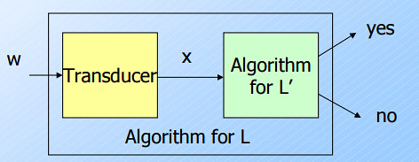
TM’s as Transducers
- We have regarded TM’s as acceptors of strings.
- But we could just as well visualize TM’s as having an output tape, where a string is written prior to the TM halting.
If we reduce $L$ to $L’$, and $L’$ is decidable, then the algorithm for $L$ + the algorithm of the reduction shows that $L$ is also decidable.
- Normally used in the contrapositive (逆否命题).
- If we know $L$ is not decidable, then $L’$ cannot be decidable.
More powerful forms of reduction: if there is an algorithm for $L’$, then there is an algorithm for $L$.
- E.g. we reduced $L_d$ to $L_u$
More in NP-completeness discussion on Karp vs. Cook reductions
- The simple reduction is called a Karp reduction.
- More general kinds of reductions are called Cook reductions.

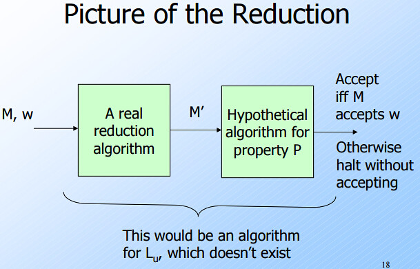
Proof of Rice’s Theorem

Proof Skeleton
- We shall show that for every nontrivial property $P$ of the RE languages, $L_P$ is undecidable.
- We show how to reduce $L_u$ to $L_P$.
- Since we know $L_u$ is undecidable, it follows that $L_P$ is also undecidable.
The Reduction
- The input to $L_u$, is a TM $M$ and an input $w$ for $M$. Then our reduction algorithm produces the code for a TM $M’$.
- Define property $P = “M \text{ accepts } w”$.
  - Thus $L(M’)$ has property $P$ if and only if $M$ accepts $w$.
    - “$L(M’)$ has property $P$” 也就意味着 “$M’$ accepts a language with property $P$”
  - That is $M’ \in L_P$ if and only if $\langle M,w \rangle \in L_u$.
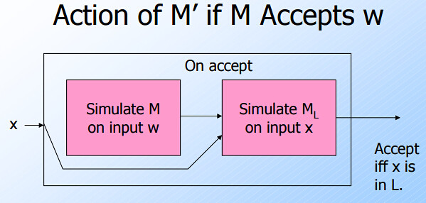
- $M’$ has two tapes, used for:
  1. Simulates another TM $M_L$ on $M’$’s own input, say $x$
    - The transducer (which in fact is $M$) does not deal with or see $x$
  2. Simulates $M$ on $w$.
    - Note: neither $M$, $M_L$, nor $w$ is input to $M’$.
- Assume that the empty language $\emptyset$ does not have property $P$.
  - If it does, consider the complement of $P$, say $Q$. $\emptyset$ then has property $Q$.
  - If we could prove that $Q$ are undecidable, then $P$ must be undecidable. That is if $L_P$ were a recursive language, then so would be $L_Q$ since the recursive languages are closed under complementation.
- Let $L$ be any language with property $P$, and let $M_L$ be a TM that accepts $L$.
Design of $M’$
1. On the second tape, $M’$ writes $w$ and then simulate $M$ on $w$.
2. If $M$ accepts $w$, then simulate $M_L$ on the input $x$ on the first tape.
3. $M’$ accepts its input $x$ if and only if $M_L$ accepts $x$, i.e. $x \in L$.
  - If $M$ does not accept $w$, $M’$ never gets to the stage where it simulate $M_L$, and therefore $M’$ accept nothing.
  - In this case, $M’$ defines an empty language, which does not have property $P$.
4. Suppose $M$ accepts $w$.
  - Then $M’$ simulates $M_L$ and therefore accepts $x$ if and only if $x$ is in $L$.
  - That is, $L(M) = L$, $L(M’)$ has property $P$, and $M’ \in L_P$.
5. Suppose $M$ does not accept $w$.
  - Then $M’$ never starts the simulation of $M_L$, and never accepts its input $x$.
  - Thus, $L(M’) = \emptyset$, and $L(M’)$ does not have property $P$.
  - That is, $M’ \not \in L_P$.
6. Thus, the algorithm that converts $M$ and $w$ to $M’$ is a reduction of $L_u$ to $L_P$.
  - Thus, $L_P$ is undecidable.

5. Turing Machines @ Erickson §6

6.1 Why Bother?

Admittedly, Turing machines are a terrible model for thinking about fast computation; simple operations that take constant time in the standard random-access model can require arbitrarily many steps on a Turing machine. Worse, seemingly minor variations in the precise definition of “Turing machine” can have significant impact on problem complexity. As a simple example (which will make more sense later), we can reverse a string of n bits in $O(n)$ time using a two-tape Turing machine, but the same task provably requires $\Omega(n^2)$ time on a single-tape machine.

But here we are not interested in finding fast algorithms, or indeed in finding algorithms at all, but rather in proving that some problems cannot be solved by any computational means. Such a bold claim requires a formal definition of “computation” that is simple enough to support formal argument, but still powerful enough to describe arbitrary algorithms. Turing machines are ideal for this purpose. In particular, Turing machines are powerful enough to simulate other Turing machines, while still simple enough to let us build up this self-simulation from scratch, unlike more complex but efficient models like the standard random-access machine.

(Arguably, self-simulation is even simpler in Church’s $\lambda$-calculus, or in Schönfinkel and Curry’s combinator calculus, which is one of many reasons those models are more common in the design and analysis of programming languages than Turing machines. Those models much more abstract; in particular, they are harder to show equivalent to standard iterative models of computation.)

6.2 Formal Definitions

Three distinct special states $\lbrace \text{start}, \text{accept}, \text{reject} \in Q \rbrace$.
A transition function $\delta: (Q \setminus \lbrace \text{start}, \text{reject} \rbrace) \times \Gamma \rightarrow Q \times \Gamma \times \lbrace −1,+1 \rbrace$.

7. Turing Machines @ Computational Complexity by Mike Rosulek

Languages and UTM (Lecture 1 & 2)

Language:

A language is a subset of $\lbrace 0,1 \rbrace^\star$ (actually it could be any subset of $\lbrace 0,1 \rbrace^\star$)
A language $L$ is a set of “yes-instances”
- $x$ is a “yes-instance” if $x \in L$
Language $S$ is Turing-recognizable (“recursively enumerable / r.e.”) if $\exists$ TM $M$, such that $\forall x$
- $x \in S \Rightarrow M$ accepts $x$
- $x \not\in S \Rightarrow M$ rejects $x$ or runs forever
Language $S$ is Turing-decidable (“recursive”) if $\exists$ TM $M$, such that $\forall x$
- $x \in S \Rightarrow M$ accepts $x$
- $x \not\in S \Rightarrow M$ rejects $x$
An algorithm formally is a TM which
1. halts on any input regardless of whether that input is accepted or not, and
2. accepts (a language) by final state
In other words, language $S$ is Turing-decidable (“recursive”) if $\exists$ an algorithm for $S$.
If $M$ is a TM, define $L(M) = \lbrace x \vert M \text{ accepts } x \rbrace$

Programming conventions:

Programming a TM for real is cruel!
Describe a TM “program” in terms of tape modifications & head movements
“Mark” cells on the tape (e.g., $a \rightarrow \acute{a}$)

E.g. TM algorithm for $\text{Palindromes} = \lbrace x \vert x = reverse(x) \rbrace$:

“Mark” first char (e.g., $O \rightarrow \emptyset$), remember that char in internal state
If char to the right is “marked” or blank, then accept; else scan right until blank or a “marked” char
If $\text{prev char} \neq \text{remembered char}$, reject; else mark it
Scan left to leftmost unmarked char; if no more unmarked chars, accept; else repeat from step #1

Universal Machines:

TMs can be encoded as strings (“code is data”)
- Convention: every string encodes some TM
- $\langle M \rangle$: encoding of a TM $M$
- $\langle M,x \rangle$: encoding of a TM $M$ and a string $x$
$L_{acc} = \lbrace \langle M,x \rangle \vert M \text{ is a TM that accepts } x \rbrace$ is Turing-recognizable (RE)
- Suppose there such a TM $U$ that accept $\langle M,x \rangle$, i.e. $U(\langle M,x \rangle) = \text{yes}$.
- $U \text{ accepts } \langle M,x \rangle \iff \langle M,x \rangle \in L_{acc}$.
- In other words, $U$ recognizes $L_{acc}$, i.e. $L(U) = L_{acc}$
TM $U$ can recognizes $L_{acc}$, which means it can simulate any TM $M$! Thus call it a “universal TM”

Design of Universal TM:

On input $\langle M,x \rangle$, use 3 tapes:
- one for description of $M$
- one for $M$’s work tape contents
- one for $M$’s current state
Transitions: $\langle \text{state, char, newstate, newchar, direction} \rangle$
Legal to say “simulate execution of $M$ on input $x$” in our TM pseudocode! – If $M$ halts on $x$, the simulation will also halt – “Simulate execution of $M$ on input $x$ for $t$ steps” also possible (always halts)
- Can simulate $t$ steps of a TM in $O(t \log t)$ steps

Diagonalization and Reduction (Lecture 2 & 3)

Diagonalization:

$L_{acc} = \lbrace \langle M,x \rangle \vert M \text{ is a TM that accepts } x \rbrace$ is not Turing-decidable (“recursive”)
- Likewise, $L_{halt} = \lbrace \langle M,x \rangle \vert M \text{ is a TM that halts } x \rbrace$
这里的 $L_{acc}$ 即前面 Jeff Ullman 的 $L_u$

(Turing) Reductions:

Motivation:
- Let’s not use diagonalization technique every time to prove something undecidable!
- Instead, “reduce” one problem to another.
What does “Alg decides lang” mean?
- Language $L = \lbrace x \vert x \text{ is/satisfies blab blah blah} \rbrace$ is a collection of yes-instances.
  - An $x$ that is/satisfies “blab blah blah” is a yes-instance.
- An algorithm is in nature a TM, so we can say “an algorithm $M$”.
- If we say “$M$ decides $L$”, it means:
  - $L(M) = L$
  - Imagine $M$ as a function,
    - The datatype of the parameter to $M$ is the the one of the elements of $L$. E.g.
      - if $L=\lbrace x \vert \dots \rbrace$, elements are $x$’s. Therefore the function signature is $M(x)$;
      - if $L=\lbrace \langle x,y \rangle \vert \dots \rbrace$, elements are $\langle x,y \rangle$’s. Therefore the function signature is $M(\langle x,y \rangle)$.
    - $M(x)=\text{yes}$ if $x$ is/satisfies “blab blah blah”
    - $M(x)=\text{no}$ otherwise
- If we say “go find an algorithm for language”, it means:
  - go find an $M$ such that $L(M) = L$
  - go find an $M$ such that $M(x)=\text{yes}$ if $x$ is/satisfies “blab blah blah”
Definition:
- We say $L_1 \leq_T L_2$ (“$L_1$ Turing-reduces to $L_2$”) if there is an algorithm that decides $L_1$ using a (hypothetical) algorithm that decides $L_2$.
Inference:
- CASE 1: implication
  - Ground Truth: $L_2$ is decidable
  - Goal: To prove $L_1$ is also decidable
  - Method: Construct an algorithm $M_1$ for $L_1$ which satisfies $L_1 \leq_T L_2$
    - $L_2$ is decidable so there must exist an algorithm $M_2$ for $L_2$
    - Call $M_2$ inside $M_1$
    - In this way we prove that $L_1 \leq_T L_2$ holds.
- CASE 2: contrapositive
  - Ground Truth: $L_1$ is undecidable
  - Goal: To prove $L_2$ is also undecidable
  - Method: Assume $L_2$ is decidable. Under this assumption, show we can construct an algorithm $M_1$ for $L_1$ which satisfies $L_1 \leq_T L_2$, i.e. $L_1 \leq_T L_2$ holds.
    - In this way we imply that $L_1$ is decidable.
    - However, we already know that $L_1$ is undecidable.
    - Therefore the assumption is invalid.
E.g. show that $L_{empty} = \lbrace \langle M \rangle \vert M \text{ is a TM and } L(M) = \emptyset \rbrace$ is undecidable.
- Choose $L_{acc} = \lbrace \langle M,x \rangle \vert M \text{ is a TM that accepts } x \rbrace$ as $L_1$
- $L_{empty}$ is $L_2$.
  - Assume there exists an algorithm $M_{empty}$.
- Construct an algorithm $M_{acc}$ using $M_{empty}$:
  - Signature: $M_{acc}(\langle M,x \rangle)$
  - For every single pair of input $\langle M_i,x_j \rangle$:
    - Construct an TM $M_{ij}^{\star}(z) = \lbrace \text{ignore } z; \text{return } M_i(x_j) \rbrace$
      - 根据 $L_{acc}$ 的语义，$M_i$ 要么 accept $x_j$，要么 reject
      - CASE 1: If $M_i$ accepts $x_j$, $M_i(x_j)=\text{yes}$.
        
        Therefore $M_{ij}^{\star}(z) = \lbrace \text{ignore } z; \text{return yes} \rbrace$.
        
        I.e. $M_{ij}^{\star}$ accept every $z$.
        
        I.e. $M_{ij}^{\star}$ accept everything.
        
        I.e. $L(M_{ij}^{\star}) = \Omega$ (全集)
        
        I.e. $\langle M_{ij}^{\star} \rangle \not \in L_{empty}$.
        
        I.e. $M_{empty}(\langle M_{ij}^{\star} \rangle) = \text{no}$.
      - CASE 2: If $M_i$ rejects $x_j$, $M_i(x_j)=\text{no}$.
        
        Therefore $M_{ij}^{\star}(z) = \lbrace \text{ignore } z; \text{return no} \rbrace$.
        
        I.e. $M_{ij}^{\star}$ rejects every $z$.
        
        I.e. $M_{ij}^{\star}$ accept nothing.
        
        I.e. $L(M_{ij}^{\star}) = \emptyset$
        
        I.e. $\langle M_{ij}^{\star} \rangle \in L_{empty}$.
        
        I.e. $M_{empty}(\langle M_{ij}^{\star} \rangle) = \text{yes}$.
    - If $M_{empty}(\langle M_{ij}^{\star} \rangle) = \text{yes}$
      - I.e. $\langle M_{ij}^{\star} \rangle \in L_{empty}$
      - 一路反推到 CASE 2，我们有 $M_i$ rejects $x_j$
      - 此时我们的 $M_{acc}(\langle M_i,x_j \rangle)$ 要 return no
    - If $M_{empty}(\langle M_{ij}^{\star} \rangle) = \text{no}$
      - I.e. $\langle M_{ij}^{\star} \rangle \not \in L_{empty}$
      - 一路反推到 CASE 1，我们有 $M_i$ accepts $x_j$
      - 此时我们的 $M_{acc}(\langle M_i,x_j \rangle)$ 要 return yes
- Now we showed $L_{acc} \leq_T L_{empty}$. We assumed $L_{empty}$ is decidable, so $L_{acc}$ is also decidable, which is against the truth. Therefore the assumption is invalid and $L_{empty}$ is undecidable.
- 最难的地方在 “Construct an algorithm $M_{acc}$ using $M_{empty}$” 这一步，请结合 $M_{acc}$ 和 $M_{empty}$ 综合考虑。一般的的套路是：
  - 根据 $L_1$ 的输入做一个临时变量，然后把这个临时变量当做 $L_2$ 的输入。
    - 这个临时变量要满足 $M_2$ 的 signature
    - 如果临时变量是一个 TM，比如上面的 $M_{ij}^{\star}$，在处理自身的输入 $z$ 时要见机行事
      - 如果能直接 $\text{return }M_i(x_j)$ 或者 $\text{return }!M_i(x_j)$ 无疑是最好的
      - 如果不能，考虑 $\text{if } M_i(x_j) = \text{yes}, \text{return } function(z)$ 这样的形式
  - 然后根据 $L_2$ 的输出决定 $L_1$ 的输出。

// Reduce L_acc to L_empty
M_acc(<M_i,x_j>) {
	M*_ij = TurningMachine(z) {
		return M_i(x_j)
	}
	
	return !M_empty(M*_ij)
}

// General form of reduction algorithm for L_acc
M_acc(<M_i,x_j>) {
	M*_ij = TurningMachine(z) {
		if(M_i(x_j) = yes) {
			return f_1(z)
		} else {
			return f_2(z)
		}
	}
	
	return f_3(M_2(M*_ij))
}

Rice’s Theorem (Lecture 4)

Rice’s Theorem. $\lbrace \langle M \rangle \vert L(M) \text{ has property } P \rbrace$ is undecidable if $P$ is non-trivial.

Non-trivial means:
- $\exists$ $M_Y$ that $L(M_Y)$ has property $P$;
- also $\exists$ $M_N$ that $L(M_N)$ does not has property $P$.
- I.e. “是否有 property $P$” 这个问题并不是永真或者永假

In other words, given encoding of $M$:

Can’t decide whether $L(M)$ is empty
Can’t decide whether some special $x \in L(M)$
Can’t decide whether $L(M)$ is finite
etc.

Define $L_P = \lbrace \langle M \rangle \vert L(M) \text{ has property } P \rbrace$.

Claim. $L_{acc} \leq_T L_P$.

Proof.

By “non-trivial”:
- Suppose $\emptyset$ does not have property $P$.
- $\exists$ $M_Y$ that $L(M_Y)$ has property $P$.
For every single pair of input $\langle M_i,x_j \rangle$, construct an TM $M_{ij}^{\star}(z)$, such that on input $z$
- If $M_i(x_j) = \text{yes}$
  - return $M_Y(z)$
- else return No
If $M_{ij}^{\star} \in L_P$, $M_{acc}(\langle M_i,x_j \rangle)$ return Yes; else No
逻辑是：
- If $M_i$ accepts $x_j$, $M_{ij}^{\star}$ 等价于 $M_Y$，此时 $M_{ij}^{\star}$ 应该具有 property $P$.
- If $M_i$ rejects $x_j$, $M_{ij}^{\star}$ 等价于 $\emptyset$，此时 $M_{ij}^{\star}$ 应该不具有 property $P$

$\blacksquare$

Kolmogorov Complexity (or, “optimal compression is hard!”) (Lecture 5 & 6) @ Algorithmic Information Theory and Kolmogorov Complexity

Problem:

假设 compress $x$ 得到 $y$，decompress $y$ 得到 $x$
假设有一个 decompression algorithm $U$ that $U(y)=x$
$K_U(x) = \min \lbrace \lvert y \rvert \vert U(y)=x \rbrace$
- How small $x$ can be compressed?
- Here $\lvert y \rvert$ denotes the length of a binary string $y$
In other words, the complexity of $x$ is defined as the length of the shortest description of $x$ if each binary string $y$ is considered as a description of $U(y)$

Optimal decompression algorithm:

The definition of $K_U$ depends on $U$.
For the trivial decompression algorithm $U(y) = y$ we have $K_U(x) = \vert x \vert$.
One can try to find better decompression algorithms, where “better” means “giving smaller complexities”

Definition 1. An algorithm $U$ is asymptotically not worse than an algorithm $V$ if $K_U(x) \leq K_V(x)+C$ for some constant $c$ and for all $x$.

Theorem 1. There exists an decompression algorithm $U$ which is asymptotically not worse than any other algorithm $V$.

Such an algorithm is described as asymptotically optimal.

The complexity $K_U$ with respect to an asymptotically optimal $U$ is called Kolmogorov complexity.
Assume that some asymptotically optimal decompression algorithm $U$ is fixed, the Kolmogorov complexity of a string $x$ is denoted by $K(x)$ ($=K_U(x)$).
- The complexity $K(x)$ can be interpreted as the amount of information in $x$ or the “compressed size” of $x$.

The construction of optimal decompression algorithm:

The idea of the construction is used in the so-called “self-extracting archives”. Assume that we want to send a compressed version of some file to our friend, but we are not sure he has the decompression program. What to do? Of course, we can send the program together with the compressed file. Or we can append the compressed file to the end of the program and get an executable file which will be applied to its own contents during the execution.
待补充。

Basic properties of Kolmogorov complexity:

待补充。

Algorithmic properties of $K$

结合 Berry Paradox 补充

Complexity and incompleteness:

不懂

Algorithmic properties of $K$ (continued):

不懂

An encodings-free definition of complexity:

不懂

Axioms of complexity:

不懂

Kolmogorov Complexity (or, “optimal compression is hard!”) (Lecture 5 & 6) @ Wikipedia

Definition

If $P$ is a program which outputs a string $x$, then $P$ is a description of $x$. The length of the description is just the length of $P$ as a character string, multiplied by the number of bits in a character (e.g. 7 for ASCII).

We could, alternatively, choose an encoding for Turing machines $\langle M \rangle$. If $M$ is a Turing Machine which, on input $w$, outputs string $x$, then the concatenated string $\langle M \rangle w$ is a description of $x$.

Any string $s$ has at least one description, namely the program:

function GenerateFixedString()
    return s

If a description of $s$, $d(s)$, is of minimal length (i.e. it uses the fewest bits), it is called a minimal description of $s$. Thus, the length of $d(s)$ (i.e. the number of bits in the description) is the Kolmogorov complexity of $s$, written $K(s)$. Symbolically, $K(s) = \vert d(s) \vert$.

Invariance theorem

Informal treatment

Theorem. Given any description language $L$, the optimal description language is at least as efficient as $L$, with some constant overhead.

Proof: Any description $D$ in $L$ can be converted into a description in the optimal language by first describing $L$ as a computer program $P$ (part 1), and then using the original description $D$ as input to that program (part 2). The total length of this new description $D’$ is (approximately): $\vert D’ \vert = \vert P \vert + \vert D \vert$.

The length of $P$ is a constant that doesn’t depend on $D$. So, there is at most a constant overhead, regardless of the object described. Therefore, the optimal language is universal up to this additive constant. $\blacksquare$

A more formal treatment

Theorem. If $K_1$ and $K_2$ are the complexity functions relative to Turing complete description languages $L_1$ and $L_2$, then there is a constant $c$ – which depends only on the languages $L_1$ and $L_2$ chosen – such that

\[\forall s, -c \leq K_1(s) - K_2(s) \leq c.\]

Proof: By symmetry, it suffices to prove that there is some constant $c$ such that for all strings $s$, $K_1(s) \leq K_2(s) + c$.

Now, suppose there is a program in the language $L_1$ which acts as an interpreter for $L_2$:

function InterpretL2(string p)
    return p()

Running InterpretL2 on input p returns the result of running p.

Thus, if $P$ is a program in $L_2$ which is a minimal description of $s$, then InterpretL2(P) returns the string $s$. The length of this description of $s$ is the sum of

The length of the program InterpretL2, which we can take to be the constant $c$.
The length of $P$ which by definition $=K_2(s)$.

This proves the desired upper bound. $\blacksquare$

Basic results

In the following discussion, let $K(s)$ be the complexity of the string $s$.

Theorem. There is a constant $c$ such that $\forall s, K(s) \leq \vert s \vert + c$.

Theorem. There exist strings of arbitrarily large Kolmogorov complexity. Formally: for each $n \in \mathbb{N}$, there is a string $s$ with $K(s) \geq n$.

Proof: Otherwise all of the infinitely many possible finite strings could be generated by the finitely many programs with a complexity below $n$ bits. $\blacksquare$

Theorem. $K$ is not a computable function. In other words, there is no program which takes a string $s$ as input and produces the integer $K(s)$ as output.

Chain rule for Kolmogorov complexity:

\[K(X,Y) = K(X) + K(Y \vert X) + O(\log(K(X,Y)))\]

It states that the shortest program that reproduces $x$ and $Y$ is no more than a logarithmic term larger than a program to reproduce $x$ and a program to reproduce $Y$ given $X$. Using this statement, one can define an analogue of mutual information for Kolmogorov complexity.

Compression

A string $s$ is compressible by a number $c$ if it has a description whose length does not exceed $\vert s \vert −c$ bits. This is equivalent to saying that $K(s) \leq \vert s \vert −c$. Otherwise, $s$ is incompressible by $c$.

A string incompressible by 1 is said to be simply incompressible––by the pigeonhole principle, which applies because every compressed string maps to only one uncompressed string, incompressible strings must exist, since there are $2^n$ bit strings of length n, but only $2^n - 1$ shorter strings.

There are $2^n$ bitstrings of length $n$. The number of descriptions of length not exceeding $n-c$ is given by the geometric series:

\[1 + 2 + 2^2 + ... + 2^{n-c} = 2^{n-c+1} - 1\]

There remain at least $2^n - 2^{n-c+1} + 1$ bitstrings of length $n$ that are incompressible by $c$. To determine the probability, divide by $2^n$.

Chaitin’s incompleteness theorem

We know that, in the set of all possible strings, most strings are complex in the sense that they cannot be described in any significantly “compressed” way. However, it turns out that the fact that a specific string is complex cannot be formally proven, if the complexity of the string is above a certain threshold.

Theorem. There exists a constant $L$ (which only depends on the particular axiomatic system and the choice of description language) such that there does not exist a string $s$ for which the statement

\[K(s) \geq L \text{(as formalized in } S \text{)}\]

can be proven within the axiomatic system $s$.

Proof by contradiction using Berry’s paradox. 略

Time/space complexity classes: P & NP @ class (Lecture 7)

Resource bounds:

$M$ has (worst case) running time $T$ if $\forall$ string $x$, $M$ halts after at most $T(\vert x \vert)$ steps.
$M$ has (worst case) space usage $s$ if $\forall$ string $x$, $M$ writes on at most $S(\vert x \vert)$ tape cells.

Basic Complexity Class:

$\text{DTIME}(f(n)) = \lbrace L \vert L \text{ decided by a (deterministic) TM with running time } O(f(n)) \rbrace$
- $\text{D}$ for “deterministic”
- Formally, $L \in TIME(f(n))$ if there is a TM $M$ and a constant $c$ such that
  1. $M$ decides $L$, and
  2. $M$ runs in time $c \cdot f$;
    - i.e., for all $x$ (of length at least 1), $M(x)$ halts in at most $c \cdot f(\lvert x \rvert)$ steps.
- E.g. $\text{DTIME}(n^2) = \text{set of all problems that can be solved in quadratic time}$
$\text{DSPACE}(f(n)) = \lbrace L \vert L \text{ decided by a TM that uses spaces } O(f(n)) \rbrace$
Language / decision problem = set of strings (yes-instances)
Complexity class = set of languages

Standard Complexity Classes:

$\text{P} = \lbrace \text{problems that can be solved (by a deterministical TM) in poly time} \rbrace$
- $\text{P} = \bigcup_{k=1,2,\dots} \text{DTIME}(n^k)$
  - 如果把 $P$ 看做 property 的话，$P$ 可以简单描述为 “deterministic poly time”
  - “deterministic” = “deterministically solvable in time” = “solvable in time by a deterministical TM”
$\text{PSPACE} = \lbrace \text{problems that can be solved using poly space} \rbrace$ $\text{PSPACE} = \bigcup_{k=1,2,\dots} \text{DSPACE}(n^k)$
$\text{EXP} = \lbrace \text{problems that can be solved by in exponential time} \rbrace$
- $\text{EXP} = \bigcup_{k=1,2,\dots} \text{DTIME}(2^{n^k})$
$\text{L} = \lbrace \text{problems that can be solved using log space} \rbrace$
- $\text{L} = \text{DSPACE}(\log n)$

Translating from “Complexity Theory Speak”:

Is $X \in \text{PSPACE}$?
- Can problem $x$ be solved using polynomial space?
Is $\text{PSPACE} \subseteq P$?
- Can every problem solvable in polynomial space also be solved in polynomial time?
This is true: $P \subseteq \text{PSPACE}$

Relationships between Complexity Classes:

$\forall f(n), \text{DTIME}(f(n)) \subseteq \text{DSPACE}(f(n))$
- This follows from the observation that a TM cannot write on more than a constant number of cells per move.
If $f(n) = O(g(n))$, then $\text{DTIME}(f(n)) \subseteq \text{DTIME}(g(n))$

Complementation @ Complement Classes and the Polynomial Time Hierarchy:

这里先声明下，全集可以表示为 $\Omega$、$\sum^{\star}$ 或者 $\lbrace 0,1 \rbrace^{\star}$
The complement of a decision problem $\mathcal{L}$, denoted $co\mathcal{L}$, is the set of “No”-instances of $\mathcal{L}$.
- 一般来说，我们可以认为 $co\mathcal{L} = \overline{\mathcal{L}} = \Omega \setminus \mathcal{L}$
- 严格来说，$\mathcal{L} \cup co\mathcal{L} = WF_{\mathcal{L}} \subseteq \Omega$ where $WF_{\mathcal{L}}$ is the set of well-formed strings describing “Yes” and “No” instances. That is, $co\mathcal{L} = WF_{\mathcal{L}} − \mathcal{L}$.
  - 只是通常会限定 $WF_{\mathcal{L}} = \Omega$
- 举个例子:Every positive integer $x>1$ is either composite (合数) or prime (质数)
  - 如果限定 $\Omega = WF_{\mathcal{L}} = \lbrace x \vert x \text{ is a positive integer and } x > 1 \rbrace$
    - $\mathcal{L} = \lbrace x \vert x \text{ is prime } \rbrace$
    - $co\mathcal{L} = \overline{\mathcal{L}} = \lbrace x \vert x \text{ is not prime }\rbrace = \lbrace x \vert x \text{ is composite }\rbrace$
  - 如果仅限定 $\Omega = WF_{\mathcal{L}} = \lbrace x \vert x \text{ is a positive integer }\rbrace$
    - $co\mathcal{L} = \overline{\mathcal{L}} = \lbrace x \vert x \text{ is not prime }\rbrace \neq \lbrace x \vert x \text{ is composite }\rbrace$
    - 因为 1 既不是 prime 也不是 composite
The complement of a complexity class is the set of complements of languages in the class.
- $\mathcal{C} = \lbrace \mathcal{L} \vert \mathcal{L} \text{ has complexity } \mathcal{C} \rbrace$
- $co\mathcal{C} = \lbrace co\mathcal{L} \vert \mathcal{L} \in \mathcal{C} \rbrace$
- 注意 $co\mathcal{C}$ 和 $\overline{\mathcal{C}}$ 没有半毛钱的关系
  - $\overline{\mathcal{C}} = \lbrace \mathcal{L} \vert \mathcal{L} \text{ does NOT have complexity } \mathcal{C} \rbrace$
  - $co\mathcal{C} = \lbrace \mathcal{L} \vert \mathcal{L} \text{‘s complement has complexity } \mathcal{C} \rbrace$
    - $\mathcal{L} \text{‘s complement has complexity } \mathcal{C}$ 并不能说明 $\mathcal{L} \text{ has } \mathcal{C} \text{ or not}$
Theorem 1. $\mathcal{C}_1 \subseteq \mathcal{C}_2 \hspace{1em} \Rightarrow \hspace{1em} co\mathcal{C}_1 \subseteq co\mathcal{C}_2$
Theorem 2. $\mathcal{C}_1 = \mathcal{C}_2 \hspace{1em} \Rightarrow \hspace{1em} co\mathcal{C}_1 = co\mathcal{C}_2$
Closure under complementation means: $\mathcal{C} = co\mathcal{C}$
- We say such class $\mathcal{C}$ are “closed under complementation”.
Theorem 3. If $\mathcal{C}$ is a deterministic time or space complexity class, then $\mathcal{C} = co\mathcal{C}$.
- E.g.
  - $co\text{TIME}(f(n)) = TIME(f(n))$
  - $coP = P$
    - 翻译一下：如果 $\mathcal{L}$ can be solved by in poly time $\Rightarrow$ $co\mathcal{L}$ can also be solved by in poly time
    - vise versa
  - $co\text{PSPACE} = \text{PSPACE}$
- Why? For any class $\mathcal{C}$ defined by a deterministic TM $M$, just switch accpet/reject behavior and you get a TM $coM$ that decide $co\mathcal{C}$
  - i.e. $M(\mathcal{L}) = \text{yes} \hspace{1em} \Rightarrow \hspace{1em} coM(co\mathcal{L}) = \text{yes}$, in the same bound of time or space.

$NP$:

$NP$ 可以描述为 nondeterministic polynomial time
- “nondeterministic” = “nondeterministically solvable in time” = “solvable in time by a nondeterministical TM”
Definition 1. A problem is assigned to the $NP$ class if it is solvable in polynomial time by a nondeterministic TM.
- $NP = \lbrace \text{problems that can be solved by a nondeterministic TM in poly time} \rbrace$
Definition 2. $NP = \text{set of decision problems } L$, where
- $L = \lbrace x \vert \exists w : M(x,w) = 1 \rbrace$
- $M$ halts in polynomial time, as a function of $\lvert x \rvert$ alone.
- $x$: instance
- $w$: proof / witness / solution
- 简单理解就是，我们没有办法直接确定是否有 $x \in L$ (nondeterministic)，只能通过 $(x,w)$ 是否满足 $L$ 的条件来判断这个 $x$ 是否有 $\in L$
举例待补充

$co\text{NP}$

Definition. $co\text{NP} = \text{set of decision problems } L$, where
- $L = \lbrace x \vert \not\exists w : M(x,w) = 1 \rbrace$
- 等价于 $L = \lbrace x \vert \forall w : M(x,w) = 0 \rbrace$
- 等价于 $L = \lbrace x \vert \forall w : M(x,w) = 1 \rbrace$
- $M$ halts in polynomial time, as a function of $\lvert x \rvert$ alone.
举例待补充

$P$ vs $NP$ vs $co\text{NP}$

Theorem 1. $P \subseteq NP$

Proof: Take any $L \in P$, then $\exists$ a PTM $M$ such that $L = \lbrace x \vert M(x) = 1 \rbrace$.

Define $M’(x,w) = \lbrace \text{ignore } w; \text{return } M(x) \rbrace$. Therefore $L=\lbrace x \vert \exists w : M,(x,w) = 1 \rbrace \in NP$ $\blacksquare$

Theorem 2. $P \subseteq co\text{NP}$

Proof: Ditto. $\blacksquare$

Closure Properties of $NP$, $co\text{NP}$

If $A, B \in \text{NP}$, then
- $A \cap B \in \text{NP}$
- $A \cup B \in \text{NP}$
If $A, B \in co\text{NP}$, then
- $A \cap B \in co\text{NP}$
- $A \cup B \in co\text{NP}$

Karp reductions, NP hardness/completeness (Lecture 8)

Karp Reduction: Define $A \leq_P B$ (“$A$ Karp-reduces to $B$”) to mean:

\[\exists \text{ poly time function } f: \quad \forall x : x \in A \iff f(x) \in B\]

$\leq_P$ is transive: $A \leq_P B \leq_P C \Rightarrow A \leq_P C$.

$L$ is $\text{NP}$-hard if $\forall A \in \text{NP} : A \leq_P L$, which means:

$L$ is at least as hard as EVERY problem in $\text{NP}$
If you could solve $L$ in poly-time then $\text{P} = \text{NP}$

$L$ is $\text{NP}$-compelte if:

$L$ is $\text{NP}$-hard
$L \in \text{NP}$

which means:

$L$ is (one of) the hardest problem in $\text{NP}$
It’s impossible to prove $\text{P} = \text{NP}$ by solving $L$ in poly-time, because $L \in \text{NP}$

Theorem. If $A \leq_P B$ and $A$ is $\text{NP}$-hard, then $B$ is $\text{NP}$-hard.

Proof: $\forall L \in \text{NP} : L \leq_P A \leq_P B \Rightarrow L \leq_P B$ $\blacksquare$

If $A \leq_P B$ and $B \in \text{P}$ $\Rightarrow A \in \text{P}$
If $A \leq_P B$ and $B \in \text{NP}$ $\Rightarrow A \in \text{NP}$
Suppose $A$ is $\text{NP}$-compelte; then $A \in P \iff \text{P} = \text{NP}$

“Canonical” NP-complete Problem $X=\lbrace \langle M,x,T \rangle \vert \exists w : M \text{ accepts } (x,w) \text{ in } \vert T \vert \text{ steps} \rbrace$.

Claim. $X \in \text{NP}$

Proof: Can be checked in poly time as a function of length of $M,x,T$ (by universal TM). $\blacksquare$

Claim. $\forall A \in \text{NP}, A \leq_P X$

Proof: $A \in \text{NP}$, so $A = \lbrace x \vert \exists w : M_A(x,w) = 1 \rbrace$ where the running time of $M_A$ is $p(\vert x \vert)$.

Define $1^{p(\vert x \vert)}$ a string of $p(\vert x \vert)$ ones. Consider $f(x)=\langle M_A,x,1^{p(\vert x \vert)}\rangle$.

$\forall x \in A : f(x) \in X$. Therefore $A \leq_P X$. $\blacksquare$

Cook-Levin Theorem & Natural NP-complete problems (Lecture 9 & 10)

Cook-Levin Theorem. $SAT = \lbrace \varphi \vert \varphi \text{ is a satisfiable boolean formula} \rbrace$ is NP-complete

How to $SAT \leq_P 3SAT$:

For a long clause in $SAT$, say $x_1 \vee x_3 \vee \overline{x_4} \vee x_2 \vee x_5$,
Introduce $s$ and break it into $(x_1 \vee x_3 \vee s) \wedge (\overline{s} \vee \overline{x_4} \vee x_2 \vee x_5)$.
- If $s$ is TRUE, then $\overline{x_4} \vee x_2 \vee x_5$ must be TRUE
- If $s$ is FALSE, then $x_1 \vee x_3$ must be TRUE
- which means, one of $x_1 \vee x_3$ and $\overline{x_4} \vee x_2 \vee x_5$ must be true
Further break into: $(x_1 \vee x_3 \vee s) \wedge (\overline{s} \vee \overline{x_4} \vee t) \wedge (\overline{t} \vee x_2 \vee x_5)$

NP in terms of nondeterministic computation (Lecture 11)

$NP = \lbrace \text{problems that can be solved by a nondeterministic TM in poly time} \rbrace$.

Nondeterministic TM:

In state $q$, reading char $c$, transition $\delta(q,c)$ is a set of possible / legal actions.
- Thus we can draw a graph of configurations for a Nondet TM on a given input $x$.
- 注意 configuration graph 不是 general 的，不是针对所有的 input $x$ 的；而是对每一个特定的 $x$，我们都可以画一个 configuration graph
- configuration graph 也可以称为 computation tree
Nondeterministic TM is just imaginary, not a realistic model for computation. Just convenient for computational theory.

Nondeterministic TM acceptance:

在 configuration tree 中，每一个 internal node（非 leaf）都是一个 configuration
- A configuration can have many outgoing edges in the configuration graph.
- 我们称每个可以走的 outgoing edge 为一个 choice
Define computation thread on $x$: a path start at $(q_{\text{start}}, x, \cdot)$
- 所以每个 computation thread 都可以看做一个 sequence of choices
Define accepting thread: a computation thread eventually reaches $(q_{\text{accept}}, \cdot, \cdot)$
NTM accepts $x$ $\iff \exists$ an accepting thread on $x$
NTM rejects $x$ $\iff \not \exists$ an accepting thread on $x$ $\iff$ all threads rejects $x$
Running time of NTM on $x$: max $\text{#}$ of steps among all threads
Space usage of NTM on $x$: max tape usage among all threads

Pitfalls of NTM:

Nondeterministic “algorithm” defined in terms of local behavior within each thread
Acceptance/rejection defined in terms of global/collective behavior of all threads
Threads can’t “communicate” with each other

$NTIME$, $NSPACE$ & $NP$

$\text{NTIME}(f(n)) = \lbrace L \vert L \text{ accepted by a NTM with running time } O(f(n)) \rbrace$
$\text{NSPACE}(f(n)) = \lbrace L \vert L \text{ accepted by a NTM that uses spaces } O(f(n)) \rbrace$
$\text{NP} = \bigcup_{k=1,2,\dots} \text{NTIME}(n^k)$

Claim: for $\text{NP}$, the witness-checking definition and the NTM definition are equivalent.

Proof: 略

Hierarchy theorems (Lecture 12 & 13)

Complexity Separations–the holy grail of computational complexity:

Containments: $P \subseteq NP, NP \subseteq PSPACE, DTIME(n) \subseteq DSPACE(n)$, etc
Separations: $P \neq NP?, P \neq PSPACE?, NP \neq coNP$?

Deterministic Hierarchy:

$\text{DTIME}(n) \subsetneq \text{DTIME}(n^2) \text{DTIME}(n^3) \dots$
$\text{DSPACE}(n) \subsetneq \text{DSPACE}(n^2) \text{DSPACE}(n^3) \dots$

How to prove $\text{DTIME}(n) \neq \text{DTIME}(n^2)$?

Better Diagonalization
略

Deterministic Time Hierarchy Theorem:

$f(n) \log f(n) = o(g(n)) \Rightarrow \text{DTIME}(f(n)) \subsetneq \text{DTIME}(g(n))$
Thus, $\text{P} \subsetneq \text{EXP}$

Deterministic Space Hierarchy Theorem:

Ditto
Thus, $\text{L} \subsetneq \text{PSPACE}$

Non-deterministic Hierarchy:

$\text{NTIME}(n) \subsetneq \text{NTIME}(n^2) \subsetneq \text{NTIME}(n^3) \dots$
$\text{NSPACE}(n) \subsetneq \text{NSPACE}(n^2) \subsetneq \text{NSPACE}(n^3) \dots$

How to prove $\text{NTIME}(n) \neq \text{NTIME}(n^2)$?

Delayed/lazy Diagonalization
略

Non-deterministic Time Hierarchy Theorem:

$f(n+1) = o(g(n)) \Rightarrow \text{NTIME}(f(n)) \subsetneq \text{NTIME}(g(n))$
Thus, $\text{NP} \subsetneq \text{NEXP}$

Non-deterministic Space Hierarchy Theorem:

Ditto
Thus, $\text{NL} \subsetneq \text{NPSPACE}$

Ladner’s theorem & NP-intermediate problems (Lecture 14)

Questions:

Most natural problems are in $P$ or $NP$-complete.
Any problem between $P$ and $NP$-complete?

Ladner’s theorem:

If $\text{P} \neq \text{NP}$ then we can construct $M^{\ast}$ such that:
- $L(M^{\ast}) \in \text{NP}$
- $L(M^{\ast}) \notin \text{P}$
- $L(M^{\ast}) \notin \text{NP}$-complete

Claim: all finite languages are in $P$.

Proof: A finite language is a finite list of all yes-instances. Build an algorithm to compare input to this list and running time is bounded. $\blacksquare$

Claim: if $L = 3SAT \setminus A$ where $A$ is finite, then $L$ is $NP$-complete.

Proof: 注意这里 $3SAT \setminus A$ 并不是表示 “infinite $3SAT$”，只是简单的表示 “$3SAT$ 抠掉了一个 finite 集合”，所以也称为 “finite modification of $3SAT$” (这里 modification 就是 exclusion 的意思)。

$3SAT \leq_P L$:

If $x \in A$ (比方说 $A$ 只有 $x_1,x_2,x_3$ 三个 literal 并只有两个 clause), convert $x$ to an instance in $L$
If $x \notin A$, $x \in L$ by definition.

$\blacksquare$

Ladner’s theorem 证明略

Polynomial hierarchy (Lecture 15)

Question:

$\text{NP}$ problem: $\lbrace x \vert \exists w : M(x, w) = 1 \rbrace$
$co\text{NP}$ problem: $\lbrace x \vert \forall w : M(x, w) = 1 \rbrace$
- $M$ runs in poly($\lvert x \rvert$) time
What about problems like $\lbrace x \vert \exists w_1 \forall w_2: M(x, w_1, w_2) =1 \rbrace$?

Polynomial Hierarchy:

Define $\Sigma_k$ problem: $\lbrace x \vert \exists w_1 \forall w_2 \cdots \square w_k: M(x, w_1, w_2, \dots, w_k)=1 \rbrace$
Define $\Pi_k$ problem: $\lbrace x \vert \forall w_1 \exists w_2 \cdots \square w_k: M(x, w_1, w_2, \dots, w_k)=1 \rbrace$
- Generally, 这里的 $M$ 应该是一个 Nondet TM
- $M$ runs in poly($\lvert x \rvert$) time
E.g.
- $\Sigma_0 = \text{P}$
- $\Sigma_1 = \text{NP}$
- $\Pi_0 = co\text{P} = \text{P}$
- $\Pi_1 = co\text{NP}$
- $\Pi_k = co\Sigma_k$
$\text{#}$ of quantifiers doesn’t matter. E.g. $L = \lbrace x \vert \forall w_1 \forall w_2 \exists w_3 \exists w_4 \exists w_5: M(x, w_1, w_2, w_3, w_4, w_5) =1 \rbrace$
- Obviously, $L \in \Pi_5$
- But also $L = \lbrace x \vert \forall (w_1,w_2) \exists (w_3, w_4, w_5): M(x, \vec{w})=1 \rbrace$, so $L \in \Pi_2$

Properties (for all $k$):

$\Sigma_k \subseteq \Sigma_{k+1} \cap \Pi_{k+1}$
$\Sigma_k \subseteq \text{PSPACE}$
$\Sigma_k = co\Pi_k$
$\Pi_k \subseteq \Sigma_{k+1} \cap \Pi_{k+1}$
$\Pi_k \subseteq \text{PSPACE}$
$\Pi_k = co\Sigma_k$

Proof of $\Sigma_k \subseteq \Sigma_{k+1} \cap \Pi_{k+1}$:

Suppose $L = \lbrace x \vert \exists w_1 \forall w_2 \cdots \exists w_k: M(x, \vec{w})=1 \rbrace \in \Sigma_k$.

Then $L = \lbrace x \vert \exists w_1 \forall w_2 \cdots \exists w_k \forall w_{junk}: M(x, \vec{w})=1 \rbrace \in \Sigma_{k+1}$ and $L = \lbrace x \vert \forall w_{junk} \exists w_1 \forall w_2 \cdots \exists w_k: M(x, \vec{w})=1 \rbrace \in \Pi_{k+1}$ $\blacksquare$

Polynomial Hierarchy:

Define $\text{PH} = \bigcup_{k=0,1,\dots} \Sigma_k = \bigcup_{k=0,1,\dots} \Pi_k$
Conjecture: for all $k > 0$: $\Sigma_k \neq \Pi_k$.
Since $\Sigma_k, \Pi_k \in \text{PSPACE}$ for all $k > 0$, we have $\text{PH} \in \text{PSPACE}$. Each $\Sigma_k$ or $\Pi_k$ is called a level in the hierarchy.

Theorem: If $\Sigma_k = \Pi_k$ for some $k$, then $\text{PH} = \Sigma_k$ (denoted as “$\text{PH}$ collapses to $k$”).

Proof: (1) If $\Sigma_k = \Pi_k$, then $\Sigma_k = \Sigma_{k+1}$.

Take any $L \in \Sigma_{k+1}$.

$L = \lbrace x \vert \exists w_1 \forall w_2 \cdots \square w_{k+1}: M(x, \vec{w})=1 \rbrace$. $M$ runs in poly time.

Using the same $M$, define $L’ = \lbrace (x,w_1) \vert \forall w_2 \exists w_3 \cdots \square w_{k+1}: M(x, \vec{w})=1 \rbrace$. Therefore $L’ \in \Pi_{k}$.

Since $\Sigma_k = \Pi_k$, $L’$ can be rewritten as $L’ = \lbrace (x,w_1) \vert \exists w_2’ \forall w_3’ \cdots \square w_{k+1}’: M(x, w_1 \vec{w}’)=1 \rbrace$.

Reconstruct $L$ using $L’$:

\[\begin{align} L &= \lbrace x \vert \exists w_1 \exists w_2' \forall w_3' \cdots \square w_{k+1}': M(x, w_1, \vec{w}')=1 \rbrace \newline &= \lbrace x \vert \exists (w_1,w_2') \forall w_3' \cdots \square w_{k+1}': M(x, w_1, \vec{w}')=1 \rbrace \in \Sigma_k \end{align}\]

(2) If $\Sigma_k = \Pi_k = \Sigma_{k+1}$, then $\Sigma_{k+1} = \Sigma_k = co\Pi_k = co\Sigma_{k+1} = \Pi_{k+1}$ $\blacksquare$

Oracle computations and a characterization of PH (Lecture 16 & 17)

Let $A$ be some decision problem and $M$ be a class of Turing machines. Then $M^A$ is defined to be the class of machines obtained from $M$ by allowing instances of $A$ to be solved in one step.

We call the “one-step” (not necessarily $O(1)$, but a guaranteed time bound) algorithm to $A$ an oracle.
E.g. we can declare an oracle to solve $3SAT$ in poly time.

Similarly, if $M$ is a class of Turing machines and $C$ is a complexity class, then $M^C = \bigcup_{A \in C} M^A$. If $L$ is a complete problem for $C$, and the machines in $M$ are powerful enough to compute polynomial-time computations, then $M^C = M^L$.

Oracle complexity classes:

Let $A$ be a decision problem, then
- $\text{P}^A = \lbrace \text{decision problems solvable by a poly-time } A\text{-OTM} \rbrace$
  - $\text{P}^A = \lbrace L(M^A) \vert M \text{ is a poly-time OTM} \rbrace$
- $\text{NP}^A = \lbrace \text{decision problems solvable by a non-det poly-time } A\text{-OTM} \rbrace$
Let $\text{C}$ be a complexity class, then
- $\text{P}^\text{C} = \bigcup_{L \in \text{C}} \text{P}^L$
  - $\text{P}^\text{C} = \lbrace \text{problems solvable by a poly-time OTM with some problem from C as its oracle} \rbrace$
- $\text{NP}^C = \bigcup_{L \in \text{C}} \text{NP}^L$
  - Differenet threads of an $\text{NP}$ computation can ask different oracle queries for $L \in \text{C}$

Note: Overloaded Notation!

$M^L$: special TM $M$ with oracle for a specific decision problem $L$
$\text{NP}^L$: complexity class $\text{NP}$ with oracle for a specific decision problem $L$
$\text{NP}^\text{C}$: complexity class $\text{NP}$ with oracle for any decision problem $\in \text{C}$

Claim: If $L$ is a $\text{C}$-complete problem, then $\text{P}^L = \text{P}^\text{C}, \text{NP}^L = \text{NP}^\text{C}$ etc.

Proof: By Karp reduction.

注意，我们的确是有 $\text{P}^\text{C} = \bigcup_{L \in \text{C}} \text{P}^L$，但是我们不要求一定要 $\exists L$ 是 $\text{C}$-complete 的。 $\blacksquare$

$\text{P}^{\text{P}} = \text{P}$
$\text{NP}^{\text{P}} = \text{NP}$
$\text{P}^{\text{NP}} = \text{P}^{co\text{NP}}$
$co\text{NP} \subseteq \text{P}^{\text{NP}}$

$\text{PH}$ new characterization:

$\Sigma_0 = \Pi_0 = \text{P}$
$\Sigma_k = \text{NP}^{\Sigma_{k-1}} = \text{NP}^{\Pi_{k-1}}$
- $\Sigma_0 = \text{P}$
- $\Sigma_1 = \text{NP}^{\text{P}} = \text{NP}$
- $\Sigma_2 = \text{NP}^{\text{NP}}$
- $\Sigma_3 = \text{P}^{\text{NP}^{\text{NP}}}$
$\Pi_{k} = co\Sigma_k$

Claim: $\Sigma_k = \text{NP}^{\Pi_{k-1}}$

Proof: By induction on $k$.

(1) [$\Sigma_k \subseteq \text{NP}^{\Pi_{k-1}}$]

Take any $L \in \Sigma_{k}$, so $L = \lbrace x \vert \exists w_1 \forall w_2 \cdots \square w_{k}: M(x, \vec{w})=1 \rbrace$. $M$ runs in poly time.

Goal: show $x \in L \Rightarrow$ $x$ is accepted by a $\text{NP}$TM $M^{\ast}$ with $\Pi_{k-1}$ oracle, i.e. $x \in L(M^{\ast})$.

Using the same $M$, define $L’ = \lbrace (x,w_1) \vert \forall w_2 \exists w_3 \cdots \square w_{k}: M(x, \vec{w})=1 \rbrace$. Therefore $L’ \in \Pi_{k-1}$.

Choose $L’$ as my oracle. Define $M^{\ast}(x)$:

Non-deterministically guess $w_1$
- 不同的 guess of $w_1$ 对应不同的一条 computation thread
Call oracle to see $(x,w_1) \stackrel{?}{\in} L’$.
Accept $x$ if oracle says yes.
- 相当于我们穷举了所有 $w_1$ 的取值，并 query $(x,w_1) \stackrel{?}{\in} L’$
- 如果有某个 query 返回了 YES，说明 $\exists$ an accepting thread $\Rightarrow$ NTM accepts $x$
- 如果所有的 query 都返回 NO，说明 $\not \exists$ an accepting thread $\Rightarrow$ NTM rejects $x$

\[\begin{align} M^{\ast} \text{ nondet accepts } x & \iff \exists \text{accepting thread on } x \newline & \iff \exists w_1 : (x, w_1) \in L' \newline & \iff \exists w_1 \forall w_2 \cdots \square w_{k}: M(x, \vec{w})=1 \newline & \iff x \in L \end{align}\]

(2) [$\Sigma_k \supseteq \text{NP}^{\Pi_{k-1}}$]

Suppose there is a $\text{NP}$TM $M^{\ast}$ using $L’ = \lbrace x \vert \forall w_2 \exists w_3 \cdots \square w_{k}: M’(x, \vec{w})=1 \rbrace \in \Pi_{k-1}$ as its oracle.

Goal: show $x \in L(M^{\ast}) \Rightarrow$ $\exists w_1: (x, w_1) \in L’’$ for some $\Pi_{k-1}$ set $L’’$.

For simplicity, assume that each thread of $M^{\ast}$ makes only 1 query to the oracle. Define an existentially quantified variable $y_1$ that include all computation threads of $M^{\ast}$.

Suppose on input $x$, $\exists$ an accepting thread of $M^{\ast}$, say $y$, that makes a query $q \stackrel{?}{\in} L’$.

CASE 1: on accepting thread $y$, oracle answer is YES.

$x \in L(M^{\ast}) \Rightarrow$ $\exists y_1: (x, y_1) \in L’$ (i.e. 我们的 $L’’$ 直接取 $L’$ 就好了).

CASE 2: on accepting thread $y$, oracle answer is NO.

$x \in L(M^{\ast}) \Rightarrow$ $\exists y_1: (x, y_1) \in coL’$

Because $coL’ \in \Sigma_{k-1}$, $\lbrace x \vert \exists y_1: (x, y_1) \in coL’ \rbrace \in \Sigma_{k-1}$ (合并 $\exists y_1$ 和 $\exists w_2$). Based on the fact that $\Sigma_{k-1} \subseteq \Sigma_{k}$, we can still conclude that $\lbrace x \vert \exists y_1: (x, y_1) \in coL’ \rbrace \in \Sigma_{k}$. $\blacksquare$

Space complexity (in terms of configuration graphs) (Lecture 18)

$\text{PSPACE} = \bigcup_{k=1,2,\dots} \text{DSPACE}(n^k)$
$\text{NPSPACE} = \bigcup_{k=1,2,\dots} \text{NSPACE}(n^k)$
$\text{L} = \text{DSPACE}(\log n)$
$\text{NL} = \text{NSPACE}(\log n)$

Configuration graphs:

Two tapes:
- Read-only input tape
- Read-write work tape (calculate space usage on this tape)
Transition: $(q, w, i, j) \rightarrow (q’, w’, i’, j’)$
- $q$: state
- $w$: content of work tape
  - Here, $\lvert w \rvert \leq$ space usage of the TM
- $i$: input tape head
- $j$: work tape head
Possible $\text{#}$ of configurations
- Suppose $M$ uses $f(n)$ space on input of length $n$
- $C_M(n) \leq \lvert Q \rvert \cdot \lvert \Gamma \rvert \cdot n \cdot f(n) = 2^{O(f(n))}$, as long as $f(n) \geq \log n$
- Note that since the input is fixed and the input tape is read-only, we do not need to consider all possible length-$n$ strings that can be written on the input tape.

Inclusions

We alread had $\text{DTIME}(f(n)) \subseteq \text{DSPACE}(f(n))$
$\text{DSPACE}(f(n)) \subseteq \text{DTIME}(2^{O(f(n))})$
$\text{NSPACE}(f(n)) \subseteq \text{NTIME}(2^{O(f(n))})$

Proof:

Let $L \in \text{DSPACE}(f(n))$. Then there is a TM $M$ that decides $L$ using $f(n)$ space. Show there is a TM $M’$ that decides $L$ in $2^{O(f(n))}$ time.

Construct $M’$ this way:

M'(x):
	run (orignal) M on x for C_M(n) steps
	if M accepted x
		return YES
	else 
		return NO

$M’$ runs in $C_M(n)$ time
If $M$ hasn’t halted in $C_M(n)$ steps, it must be in an infinite loop

$\blacksquare$

$\text{PSPACE}$-completeness (Lecture 18 & 19)

Canonical $\text{PSPACE}$-complete problem:

$X=\lbrace \langle M,x,1^s \rangle \vert M \text{ is a DTM that accepts } x \text{ using } \leq s \text{ space}\rbrace$

To prove that $L$ is $\text{PSPACE}$-complete:

Show that $L \in \text{PSPACE}$
If $L \in \text{PSPACE}$, then $L$ is decided by some TM $M$ that uses $s(n)$ space. Show $X \leq_P L$ via $f(x) = \langle M,x,1^{s(n)} \rangle$
- $x \in L \iff f(x) \in X$

TQBF

$TQBF$ is $\text{PSPACE}$-complete
- 证明待补充
$TQBF$ is also $\text{NPSPACE}$-complete
So $\text{PSPACE} = \text{NPSPACE}$

Geography Game

What does “Play 1 has winning strategy” mean?
- $\exists$ winning trategy, 所以 Play 1 是不能乱走的，是 $\exists$ winning moves，但是你得下出来才行
- 那对 Player 2 而言，你无论怎么下都是输，所以是 $\forall$ moves of Player 2
后略

Regex Universality

Connectivity problems / Savitch’s theorem (Lecture 20)

$\text{L} = \text{DSPACE}(\log n)$
$\text{NL} = \text{NSPACE}(\log n)$
$\text{L} \subseteq \text{NL}$
$\text{NL} \subseteq \text{NPSPACE}$

$\text{NL}$-completeness

Karp reductions don’t make sense for defining $\text{NL}$-completeness
Define log-space reduction $A \leq_L B$:
- $\exists$ a log-space computable function $f$ such that $x \in A \iff f(x) \in B$
- What does “log-space computable function” mean?
  - $f$ requires $O(\log n)$ memory to be computed
    - This restriction does NOT apply to the size of output
  - The TM computating $f$ has:
    - read-only input tape
    - unidirectional output tape (“write-once”)
    - $O(\log n)$-length read/write work tape
      - TM cannot “cheat” and use output tape as storage

$CONN = \lbrace (G,s,t)\vert G \text{ is a directed graph with a directed path from } s \text{ to } t \rbrace$

Assume $G$ is represented by an adjacency matrix
Vertices are named $1,2,\dots,n$
- It takes $O(\log n)$ bits to write a single vertex name
- Log-space is only enough to store $O(1)$ number of vertex names

Claim: $CONN$ is $\text{NL}$-complete

Proof:

(1) $CONN \in \text{NL}$

Idea: start from $s$, nondet guess to $t$

CONN(G, s, t):
	_curr = s
	
	for i = 1 to n:
		guess _next from {1,2,...,n}
		
		if no _curr → _next edge:
			reject
		if _next == t:
			accept
			
		_curr = _next
	
	reject

Scan adjacency matrix cells one by one to detect _curr → _next edge
2 variables: _curr and _next $\Rightarrow 2 \log n$ space

(2) $CONN$ is $\text{NL}$-hard

Reduction strategy: Let $M$ be a $\text{NL}$ machine. On input $x$, output $\langle G,s,t \rangle$ so that $M$ accepts $x \iff \exists s \rightsquigarrow t$ path in $G$.

Idea:

Let $G$ be the configuration graph of $M$ on $x$
$s$ be the start configuration
$t$ be the (unique) accepting configuration

Each configuration can be represented using $O(\log n)$ bits, and the adjacency matrix can be generated in log-space as follows (matrix 本身要 $O(n^2)$ space，但是这是 output 的 size，并不受 log-space 的限制):

for each configuration i:
	for each configuration j:
		Output 1 if there is a legal transition from i to j, and 0 otherwise
		(if i or j is not a legal state, simply output 0)

The algorithm requires $O(\log n)$ space for i and j, and to check for a legal transition. $\blacksquare$

Corollary: $\text{NL} \subseteq \text{P}$

Proof: Take any $A \in \text{NL}$. Because $CONN$ is $\text{NL}$-complete, there must exists a log-space function $f$ that for every input $x$ to $A$, $f(x) = \langle G,s,t \rangle$ and $x \in A \iff \exists s \rightsquigarrow t$ path in $G$.

We can construct an algorithm for $A$ using poly time:

A(x):
	run BFS on f(x) to see whether exists s → t path

So $A \in \text{P}$. $\blacksquare$

Summary:

$\text{L} \subseteq \text{NL} \subseteq \text{P} \subseteq \text{NP} \subseteq \text{PSPACE} \subseteq \text{EXP}$
By the hierarchy theorems (and Savitch’s theorem, below) we know $\text{NL} \subset \text{PSPACE}$, and $\text{P} \subset \text{EXP}$. But we cannot prove that any of the inclusions above is strict.

Claim: $CONN \in \text{DSPACE}(\log^2 n)$

Proof: Define a recursive algorithm Path(a,b,i) to seek “is there a $a \rightsquigarrow b$ path whose length $\leq 2^i$?”

Path(a,b,i):
	if i == 0:
		check (a,b) edge in adjacency matrix
	else:
		for each vertex v
			if Path(a,v,i-1) && Path(v,b,i-1)
				accept
		
		reject

Call Path(s, t, log n) to check $\langle G,s,t \rangle$
Space Usage
- depth of recursion: $\log n$
- stack frame of each iteration: space to write down a,b,i,v $\Rightarrow O(\log n)$
- Totally: $\log n \times O(\log n) = O(\log^2 n)$

$\blacksquare$

Savitch’s theorem: $\text{NSPACE}(s) \subseteq \text{DSPACE}(s^2)$ (for $s > log(n)$)

Implies that “Nondeterminisim saves at most quadratic amount of space”

Proof: 待续 $\blacksquare$

Corollary 7: If $s(n) \geq \log n$ is space constructible, then $\text{NSPACE}(s(n)) = co\text{NSPACE}(s(n))$.

Corollary 8: $\text{NL} = co\text{NL}$.

参 Katz §7

Counting complexity / $\text{#P}$ / $\text{#P}$-completeness / Parsimonious Reductions (Lecture 21)

Complexity of Counting:

So far in the class: decision problems
This unit: counting problems

Counting complexity classes $\text{FP}$, $\text{#P}$

For this lecture, “function” means $f : \lbrace 0,1 \rbrace^{\ast} \mapsto \mathbb{N}$ ($\mathbb{N}$ for “Natural number”)
$\text{FP} = \lbrace \text{functions computable in deterministically poly time} \rbrace$
If $M$ is a Nondet TM, define: $\text{#M}(x)=\text{number of accepting threads of } M \text{ on input } x$
- 注意这是一个 function，不是一个 decision problem
- 这个 function 即是一个 counting problem
- 实际应用时，$M$ 可以是一个 problem，e.g. $\text{#SAT}$: given boolean formula $\phi$, determine $\text{#}$ of satisfying assignments of $\phi$
$\text{#P} = \lbrace \text{#M} \vert M \text{ is a Nondet poly-time TM} \rbrace$
- $\text{#P} = \lbrace \text{functions that count # of accepting threads of a NTM} \rbrace$
- A function $f : \lbrace 0,1 \rbrace^{\ast} \mapsto \mathbb{N}$ is $\in \text{#P}$ if $\exists$ a TM $M$ running in poly time such that $f(x) = \text{#M}(x)$

Claim: $\text{FP} \subset \text{#P}$

Proof: Idea: given $f \in \text{FP}$, design a poly-time NTM $M$ that $\text{#M}(x) = f(x)$.

M(x):
	compute f(x) # in poly time
	nondet guess positive integer i
	accept if i <= f(x)

In this way, $i = 1,2,\dots,f(x)$ will be accepted, thus $f(x)$ accepting thread.

优化策略：searching space 可能会很大，比如 $f(x)=10$，你却在 $1,\dots,99999$ 的范围内 guess。此时你可以限制 guess 的 $i$ 不超过 $f(x)$ 的 bit 数。 $\blacksquare$

Claim: $\text{#P}$ is closed under addition & multiplication

Proof: Equal to prove $f,g \in \text{#P} \Rightarrow f+g \in \text{#P}$ and $f \ast g \in \text{#P}$

Let

$f(x)$ $\text{#}$ accepting threads of $M_f$ on $x$
$g(x)$ $\text{#}$ accepting threads of $M_g$ on $x$

(1) $f+g \in \text{#P}$

Define $M_{f+g}$

M_fg(x):
	nondet guess bit b
	if b == 0:
		return M_f(x)
	else:
		return M_g(x)

相当于把 $M_f(x)$ 和 $M_g(x)$ 这两棵 computation tree 的 root 连接到一个新的 root 上，称为一棵新的 computation tree。

(2) $f \ast g \in \text{#P}$

Define $M_{f \ast g}$

M_fg(x):
	run M_f(x)
	if M_f(x) reached an accepting thread
		return M_g(x)

相当于把 $M_f(x)$ 的 computation tree 的每一个 leaf 上连接一棵 $M_g(x)$ 的 computation tree。$\blacksquare$

Claim: if $\text{FP} = \text{#P}$ then $\text{P} = \text{NP}$

Proof: Already known that $\text{#SAT} \in \text{#P}$, so if $\text{FP} = \text{#P}$, $\text{#SAT} \in \text{FP}$.

$\text{NP}$-complete problem $SAT$ can be solved in poly time by running $\text{#SAT}(x)$ and see if the result $>0$. $\blacksquare$

$\text{#P}$-hardness

Not equivalent definitions, but both commonly used
- Def. 1: $f$ is $\text{#P}$-hard if a poly time algorithm for $f$ implies $\text{#P} = \text{FP}$ (thus $\text{P} = \text{NP}$)
- Def. 2: $f$ is $\text{#P}$-hard if $\forall g \in \text{#P}, g \leq_1 f$ via a parsimonious reduction

Parsimonious Reduction

Let $g$ & $f$ be counting problems (functions)
$g \leq_1 f$ if there $\exists$ a poly-time function $h$ such that $\forall x, f(h(x)) = g(x)$

Claim: if $g \leq_1 f$ and $f \in \text{FP}$, then $g \in \text{FP}$

Claim: The counting version of any $\text{NP}$-complete problem is $\text{#P}$-complete, i.e. if $M$ is a NTM where $L(M)$ is $\text{NP}$-complete, then $\text{#M}$ is $\text{#P}$-complete.

Proof: Use $\text{#P}$-hardness definition 1.

If $\text{#M} \in \text{FP}$, I can solve $L(M)$, a $\text{NP}$-complete problem in poly time by computing whether $\text{#M}(x) > 0$. $\blacksquare$

Claim: $\text{#SAT}$ is $\text{#P}$-complete

Proof: Use $\text{#P}$-hardness definition 2.

Given arbitrary $M$ and $x$, construct formula $\phi$ such that $\exists w : M(x,w) = 1 \iff \phi \text{ is satisfiable}$.

Let $f(w) = \text{#} w \text{ that } M(x,w) = 1$. Obviously,

$f \in \text{#P}$ and $f$ can represent $\forall \cdot \in \text{#P}$
$f(w) = \text{#SAT}(\phi)$.

$\Rightarrow \text{#SAT}$ is $\text{#P}$-hard. $\blacksquare$

待续。 Katz §23 需要大量补充进来

$\text{#P}$-completeness of the permanent (Lecture 22)

暂略

Randomized complexity classes / Amplification (Lecture 23)

2 ways to define a randomized TM (以下综合 slides、Katz §12 和 Trevisan §5.1):

[“Lazy”] Deterministic TM with two transitions functions
- A random one is applied at each step
[“Upfront”] Deterministic TM with an additional read-only “random tape”
- Each cell of this random tape is initialized randomly (with 0/1)
  - Only finite portion of this random tape can actually be used
Randomized TM $M(x;r)$ 你看做接受两个输入比较好理解：
- For a fixed $x$, $M(x;r)$ is the deterministic result with random choices $r$
- Then what is $r$?
  - [“Lazy”] The $i^{\text{th}}$ bit of $r$ determines which transition function is used at the $i^{\text{th}}$ step
  - [“Upfront”] $r$ is the value written on $M$’s random tape.
  - 也就是说，给定 $x$，我们在穷举 $r = r^{(1)},r^{(2)} \dots$:
    - 对某些 $r^{(i)}$，$M(x;r^{(i)}) = 1$
    - 对某些 $r^{(j)}$，$M(x;r^{(j)}) = 0$
    - 这样一来就存在一个 frequency 即 $\frac{\text{# } r^{(i)} : M(x;r^{(i)}) = 1}{\lvert r \vert}$。概率就这么出来了。
    - 如果你给了一个新的 $x’$，那么会有一组新的 $r^{(i’)}$ 和 $r^{(j’)}$，概率也会不同
      - 也就是说，同一个 $r^{(i)}$ 值，不一定有 $M(x;r^{(i)}) = M(x’;r^{(i)})$
- How long is $r$? I.e. $\lvert r \vert = ?$
  - $\lvert r \vert$ is polynomial in the input length $\lvert x \vert$
- 如果给定 $x$，把 $r$ 看做一个变量，那么 $M(x)$ 即是一个 distribution induced by uniform $r$
  - 你也可以把 $M(x)$ 看做是一个 Nondet TM，每一个 $r^{(i)}$ 对应一条 computation thread
Randomized TM $M(x;r)$ runs in poly time (poly in $\lvert x \vert$)
- 这个很好理解，因为 $\textbf{RT} = \text{# of steps} = \lvert r \rvert = p(\lvert x \rvert)$

PPT = probabilistic, polynomial-time

An algorithm $A$ is probabilistic polynomial time (PPT) if it uses randomness (i.e, flips coins) and its running time is bounded by some polynomial in the input size.
Alternatively, “expected poly time” means $\exists$ a polynomial (这里指 “多項式”) $p()$ such that $\mathrm{E}[\text{# of steps}] = p(\lvert x \rvert)$

$\text{RP}$ = Randomized Poly-time

$\text{RP}$ = languages $L$ of the form:
- $x \in L \Rightarrow \Pr[M(x) = 1] \geq \frac{1}{2}$ ($M$ is a PPT TM, hereafter)
- $x \not \in L \Rightarrow \Pr[M(x) = 0] = 1$
  - 注意：$x \in L$ 时的 $M(x)$ 和 $x \not \in L$ 时的 $M(x)$ 是两套不同的 distribution，所以 $x \in L$ 时的 $\Pr[M(x) = 1]$ 和 $x \not \in L$ 时的 $\Pr[M(x) = 0]$ 没有任何关系，相加也不为 1。这个概念完整点写是这样的：
    - $x \in L \Rightarrow \Pr[M(x) = 1] \geq \frac{1}{2}$ (同时 $\Pr[M(x) = 0] \leq \frac{1}{2}$)
    - $x \not \in L \Rightarrow \Pr[M(x) = 0] = 1$ (同时 $\Pr[M(x) = 1] = 0$)
换个角度陈述：$L \in \text{RP}$ if $\exists$ a PPT TM $M$ such that:
- $x \in L \Rightarrow \Pr[M(x) = 1] \geq \frac{1}{2}$
- $x \not \in L \Rightarrow \Pr[M(x) = 0] = 1$
Trevisan §5.1 的表述更好理解：$L \in \text{RP} \iff \exists$ a PPT TM $M$ and a polynomial $p()$ such that:
- $\forall x \in L : \Pr_{r\in \lbrace 0,1 \rbrace^{p( \lvert x \rvert)}}[M(x;r) = 1] \geq \frac{1}{2}$
- $\forall x \not \in L : \Pr_{r\in \lbrace 0,1 \rbrace^{p( \lvert x \rvert)}}[M(x;r) = 1] = 0$
$\text{RP}$ has one-sided error.

题外话：我们还可以类似地定义 $\text{P}$:

$L \in \text{P} \iff \exists$ a PPT TM $M$ and a polynomial $p()$ such that:
- $\forall x \in L : \Pr_{r\in \lbrace 0,1 \rbrace^{p( \lvert x \rvert)}}[M(x;r) = 1] = 1$
- $\forall x \not \in L : \Pr_{r\in \lbrace 0,1 \rbrace^{p( \lvert x \rvert)}}[M(x;r) = 1] = 0$

Claim: $\Pr[M(x) = 1] \geq \frac{1}{2}$ 里的 $\frac{1}{2}$ is not fundamental to this definition.

Explaination: I can always “amplify” $M$ to a new PPT $M’$:

def M'(x):
	run M(x) independently t times
	accept if any trial accepts

\[\begin{align} x \in L &\Rightarrow \Pr[M'(x) = 1] = 1 - \Pr[M'(x) = 0] \geq 1 - (\frac{1}{2})^t = 1 - \frac{1}{2^t} \newline x \not \in L &\Rightarrow \Pr[M'(x) = 0] = 1^t = 1 \end{align}\]

注意 $x \in L$ 时的 $\Pr[M’(x) = 0]$ 不等于 $x \not \in L$ 时的 $\Pr[M’(x) = 0]$. $\blacksquare$

所以 $\Pr[M(x) = 1] \geq \frac{1}{2}$ 里的 $\frac{1}{2}$ 其实可以是任意的 $\frac{1}{t}$。这个 amplification 更大的意义在于，如果我在多次试验 $M(x)^{(1)},M(x)^{(2)},\dots,M(x)^{(n)},\dots$ 中:

只要有一次 $M(x)^{(i)} = 1$，我就可以 100% 判断 $x \in L$
- 我们称这个判断为 “no false positive”，i.e. 只要是判断为 positive 的（i.e. 判断 $x \in L$），一定是 true positive（i.e. 与 ground truth 吻合）。
- 同理，$co\text{RP}$ 是 “no false negative”.
一次 $M(x)^{(i)} = 0$ 无法判断一定有 $x \not \in L$

注：写上面两段话时，我还没有领悟到 Trevisan §5.1 的概念更好理解。我自己写的 $M(x)^{(i)}$ 其实就是 $M(x;r^{(i)})$。

注二：Trevisan §5.1 的概念同时也跟方便理解 “什么是 error”？

我们期待的效果是像 $\text{P}$ 一样：
- $\forall x \in L : \Pr_{r\in \lbrace 0,1 \rbrace^{p( \lvert x \rvert)}}[M(x;r) = 1] = 1$
- $\forall x \not \in L : \Pr_{r\in \lbrace 0,1 \rbrace^{p( \lvert x \rvert)}}[M(x;r) = 1] = 0$
实际情况达不到的话，假设：
- $\forall x \in L : \Pr_{r\in \lbrace 0,1 \rbrace^{p( \lvert x \rvert)}}[M(x;r) = 1] \geq a$
- $\forall x \not \in L : \Pr_{r\in \lbrace 0,1 \rbrace^{p( \lvert x \rvert)}}[M(x;r) = 1] \leq b$
那么 error 可以这么计算：
- $x \in L$-side error = $1-a$
- $x \not \in L$-side error = $b-0$ = $b$
这样就很好理解 $\text{RP}$ 的 one-sided error
下面的 $\text{BPP}$ 是 2-sided error；而且两边 error 相等，i.e. $a+b=1$
- 我们可以笼统地称 $\text{BPP}$ 的 error = $1-a$，即不用特定指是哪一边。

$\text{BPP}$ = Bounded Probabilistic Poly-time

$\text{BPP}$ = languages $L$ of the form:
- $x \in L \Rightarrow \Pr[M(x) = 1] \geq \frac{2}{3}$
- $x \not \in L \Rightarrow \Pr[M(x) = 0] \geq \frac{2}{3}$
Trevisan §5.1 的表述更好理解：$L \in \text{BPP} \iff \exists$ a PPT TM $M$ and a polynomial $p()$ such that:
- $\forall x \in L : \Pr_{r\in \lbrace 0,1 \rbrace^{p( \lvert x \rvert)}}[M(x;r) = 1] \geq \frac{2}{3}$
- $\forall x \not \in L : \Pr_{r\in \lbrace 0,1 \rbrace^{p( \lvert x \rvert)}}[M(x;r) = 1] \leq \frac{1}{3}$
$\text{BPP}$ has 2-sided error

How to amplify $\text{BPP}$ algorithm?

def M'(x):
	run M(x) independently t times
	take the majority output

Chernoff Bound: How to calculate $x \in L \Rightarrow \Pr[M’(x) = 1]=?$

IID
- 我们总说是 independent and identically distributed random variables，换个方法断句可能更好理解一些：identically distributed, independent r.v.
- 假设有这么一个试验：在单次试验 $X^{(i)}$ 中，我们要抛 $t$ 次硬币，分别得到 $X_1^{(i)},X_2^{(i)},\dots,X_n^{(i)}$ 这 $t$ 个结果
- 执行 $n$ 次试验，我们可以得到 $t$ 组值，分别是 $\lbrace X_1^{(1)},\dots,X_1^{(n)} \rbrace, \lbrace X_2^{(1)},\dots,X_2^{(n)} \rbrace, \dots, \lbrace X_t^{(1)},\dots,X_t^{(n)} \rbrace$。
- 于是这 $t$ 组值构成 $t$ 个 distribution，也就是 $t$ 个 r.v. $X_1,X_2,\dots,X_t$
  - 这 $t$ 个 r.v. 是 identical 的。在这里抛硬币的例子里，大家都是 Bernoulli；不可能 $X_1$ 是 Bernoulli 然后 $X_2$ 是 Gaussian.
  - 这 $t$ 个 r.v. 是 independent 的。明显，第一次抛并不会影响第二次抛。

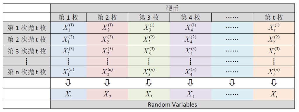
Suppose $X_1,X_2,\dots,X_t$ are IID and $\Pr[X_i = 1] = p$ (this is how they are “identical”), then Chernoff Bound states that $\Pr[\sum X_i > (1+\epsilon)tp] < \exp(-\frac{tp}{2}\epsilon^2)$.
- 简单理解就是，$\Pr[\text{total # of heads I observed} \ggg \text{total # of heads I expected}]$ is exponentially small
- 这个其实就是 quantile 的理论，见下图

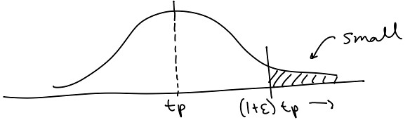
我们回头算 $\text{BPP}$ 的 amplification:

Suppose $X_i$ is the event of “obtaining wrong answer in $i^{\text{th}}$ trial of $M(x)$”, so $\Pr[Xi] \leq \frac{1}{3}$.
Let $\epsilon = \frac{1}{2}$ and $tp = \frac{t}{3}$

\[\begin{align} \Pr[\text{majority gives wrong answer}] &= \Pr \big [\sum X_i > \frac{t}{2} \big ] \newline & = \Pr \big [\sum X_i > (1+\epsilon)tp ] \newline & < \exp(-\frac{tp}{2}\epsilon^2) \newline & = \exp(-\frac{t}{24}) \end{align}\]

Let $t = 24 \lvert x \rvert$ and then
- $x \in L \Rightarrow \Pr[M(x) = 1] \geq 1 - e^{-\lvert x \rvert}$
- $x \not \in L \Rightarrow \Pr[M(x) = 0] \geq 1 - e^{-\lvert x \rvert}$

Katz §12 很精彩，值得一看

Relations between randomized complexity classes (Lecture 24)

$\text{PP}$ = Probabilistic Poly-time

$L \in \text{PP} \iff \exists$ a PPT TM $M$ and a polynomial $p()$ such that:
- $\forall x \in L : \Pr_{r\in \lbrace 0,1 \rbrace^{p( \lvert x \rvert)}}[M(x;r) = 1] > \frac{1}{2}$
- $\forall x \not \in L : \Pr_{r\in \lbrace 0,1 \rbrace^{p( \lvert x \rvert)}}[M(x;r) = 1] \leq \frac{1}{2}$
$\text{PP}$ is unrealistic
$\text{PP}$ cannot be amplified

Lemma. $L \in \text{BPP} \Rightarrow \exists$ a PPT TM $M$ with error $\leq \frac{1}{\lvert r \rvert}$

证明我就不详说了，反正一定可以 amplify 到。这个 Lemma 主要是为了证明 Sipser-Lautemann Theorem 服务的。

Sipser-Lautemann Theorem: $\text{BPP} \in \Sigma_2 \cap \Pi_2$

Proof: $\text{BPP}$ is closed under complement, i.e. $\text{BPP} = co\text{BPP}$.

所以一旦我们证明了 $\text{BPP} \in \Sigma_2$，马上就能得到 $\text{BPP} = co\text{BPP} \in \Pi_2$。得证。

下面我们全力证明 $\text{BPP} \in \Sigma_2$。

暂略。 $\blacksquare$

Non-uniformity in terms of circuits & advice / $\text{P/poly}$ (Lecture 25)

Question: Does it help to have a different algorithm for each input length?

Non-uniformity

TM is a “uniform” model of computation–a single TM handles all inputs.
A circuit only handle input with a fixed length.

Circuits

A circuit $C_n$ has $n$-bit input and is constructed with AND gates, OR gates and NOT gates.
A circuit $C_n$ computes a function $f_C : \lbrace 0, 1 \rbrace^n \mapsto \lbrace 0, 1 \rbrace$
Define $SIZE(C_n)=\text{# of gates in } C_n$ and $DEPTH(C_n)=$max path length from input to output
Define Circuit family $C = \lbrace C_1, C_2, \dots \rbrace$
- $C_i$ has $i$-bit input
- $C$ accepts $x$ if $C_{\lvert x \rvert}(x) = 1$
- $L(C) = \lbrace x \vert C \text{ accepts } x \rbrace$
  - i.e. $L$ is decided by $C$ $\iff \forall x \in L, C_{\lvert x \rvert}(x) = 1$
- Size of $C$ is $f(n)$ such that $\forall C_i \in C, SIZE(C_i) \leq f(i)$

$\text{PSIZE}$

$\text{SIZE}(f(n)) = \lbrace$ decision problems accepted by circuit family of size $f(n)\rbrace$
$\text{PSIZE} = \bigcup_{c>0} \text{SIZE}(n^c)$

Claim: Every language (even undecidable) is in $\text{SIZE}(O(2^n))$

Proof: Suppose $x \in L$ and $\lvert x \rvert = n$. Thus $x = x_1 x_2 \dots x_n$.

Use the identity $f(x_1 x_2 \dots x_n) = (x_1 \wedge f(1 x_2 \dots x_n)) \vee (\overline{x_1} \wedge f(0 x_2 \dots x_n))$ to recursively construct a circuit for $f$.

The size of the circuit is: $s(n) = 3 + 2s(n−1)$ with base case $s(1) = 1$, which solves to $s(n) = 2 \times 2^n − 3 = O(2^n)$. $\blacksquare$

注意解题技巧：我们这里说的 $n$，其实都是 $\lvert x \rvert$，所以你上来一个 $x \in L$ 其实都是包含了 $\lvert x \rvert = n$。

Relationship between $\text{P}$, $\text{NP}$, $\text{PSIZE}$

$\text{P} \subset \text{PSIZE}$
Possibly $\text{NP} \not \subseteq \text{PSIZE}$

Theorem (Cook-Levin) Take any poly-time TM $M$. $M$’s behavior on input of length $n$ can be written as a poly-size circuit. I.e. $\text{P} \subseteq \text{PSIZE}$

注：$\text{P} \neq \text{PSIZE}$ 需要另外证明

Theorem (Karp-Lipton-Sipser) If $\text{NP} \subseteq \text{PSIZE}$ then $\text{PH} = \Sigma_2$

$\text{P/}f(n)$: poly-time with $f(n)$-bounded advice

Definition: $L \in \text{P/}f(n) \iff \exists$ a poly-time TM $M$ such that $\forall n$, $\exists$ an advice string $a$ with $\lvert a \rvert = f(n)$ and $M(x,a) = 1 \forall x \in L$

注意：这里是 $\forall n \exists a$ 不是 $\forall x \exists a$。也就是说，所有的 $x$ with $\lvert x \rvert = n$ 用的是同一个 $a$，而不是每个 $x$ 都配一个。

你可以想象成有一个 advice pool $A = \lbrace a_1,a_2,\dots \rbrace$ where $\lvert a_n \rvert = f(n)$ and $x \in L, \lvert x \rvert = n \Rightarrow M(x, a_n) = 1$

$\text{P/}1$ = problems solvable with a 1-bit advice
$\text{P/}n^2$ = problems solvable with a $n^2$-bit advice
$\text{P/}poly$ = problems solvable with a $p(n)$-bit advice

Claim: $\text{P/}poly = \text{PSIZE}$

Proof:

(1) $\text{P/}poly \supseteq \text{PSIZE}$

Take any $L \in \text{PSIZE}$. Then $\exists$ a circuit family $C = \lbrace C_1, C_2, \dots \rbrace$ such that $\forall x \in L, C_{\lvert x \rvert}(x) = 1$.

Let $a_{\lvert x \rvert}$ be the description of $C_{\lvert x \rvert}$. Define TM:

def M(x, a_n):
	interpret a_n as circuit
	evaluates it on x

$M$ runs in poly-time. Therefore $x \in L \iff M(x, a_{\lvert x \rvert}) = 1$, i.e. $L \in \text{P/}poly$, i.e. $\text{P/}poly \supseteq \text{PSIZE}$.

(2) $\text{P/}poly \subseteq \text{PSIZE}$

Take any $L \in \text{P/}poly$. Then $\exists$ a poly-time TM $M$ and a set of advices $A = \lbrace a_1, a_2, \dots \rbrace$ such that $\forall x \in L, M(x, a_{\lvert x \rvert}) = 1$.

According to Theorem (Cook-Levin), any poly-time TM can be written as a poly-size circuit, so define $C_{\lvert x \rvert}$ to be the circuit with the same behavior as $M(x, a_{\lvert x \rvert}) = 1$. Thus $L \in \text{PSIZE}$, i.e $\text{P/}poly \subseteq \text{PSIZE}$. $\blacksquare$

Karp-Lipton theorem / Meyer’s theorem (Lecture 26)

Karp-Lipton theorem If $\text{NP} \subseteq \text{P/}poly$, then $\text{PH} = \Sigma_2$

Idea: First use $\text{SAT} \in \text{NP} \Rightarrow \text{SAT} \in \text{P/}poly$.

Then use $\Pi_2 \text{SAT} \in \Pi_2$. Note that $\Pi_2 \text{SAT}$ is $\Pi_2$-complete. Prove $\Pi_2 \text{SAT} \in \Sigma_2$.

Proof: If $\text{SAT} \in \text{P/}poly$, then $\exists$ a circuit family $C = \lbrace C_1, C_2, \dots \rbrace$ of poly size such that $\phi$ is satisfiable $\Rightarrow C_{\lvert \phi \rvert}(\phi) = 1$

$\Pi_2 \text{SAT} = \lbrace \phi \vert \forall y \exists z : \phi(y,z) = 1 \rbrace$

\[\begin{align} \phi \in \Pi_2 \text{SAT} & \iff \forall y \exists z : \phi(y,z) = 1 \newline & \iff \forall y : \phi(y,\cdot) = 1 \newline & \iff \forall y : C_{\lvert \phi(y,\cdot) \rvert}(\phi(y,\cdot)) = 1 \newline & \iff \exists C_{\lvert \phi(y,\cdot) \rvert} \forall y : C_{\lvert \phi(y,\cdot) \rvert}(\phi(y,\cdot)) = 1 \end{align}\]

So $\Pi_2 \text{SAT} \in \Sigma_2$, i.e. $\text{PH} = \Sigma_2$. $\blacksquare$

Meyer’s theorem If $\text{EXP} \subseteq \text{P/}poly$, then $\text{EXP} = \Sigma_2$

Note: Weird sequences:

$\text{EXP}$ is closed under complememt. Therefore if $\text{EXP} = \Sigma_2$, then also $\text{EXP} = co\text{EXP} = \Pi_2 \Rightarrow \text{PH} = \Sigma_2$
Already known that $\text{P} \neq \text{EXP}$ by time hierarchy theorem $\Rightarrow \text{P} \neq \Sigma_2 \Rightarrow \text{P} \neq \text{NP}$

Proof: Given $L \in \text{EXP}$ decided by TM $M$, define

$ST(x,t)$: On input $x$, $M$ is in this state after $t$ steps
$HD(x,t)$: On input $x$, $M$’s tape head is at this index after $t$ steps
$TP(x,t,i)$: On input $x$, $M$’s tape has this character at index $i$ after $t$ steps
- $t, i$ are numbers $\leq 2^{p(n)}$ (because of $\text{EXP}$), so required $p(n)$ bits to write them down
- Suppose the maximum step number is $t_{max}$

$M$ accepts $x \iff ST(x, t_{max}) = q_{accept}$.

We can imagine $ST$, $HD$ and $TP$ as 3 circuits. They must be consistent with $M$’s transition function and tape cells. We can check the consistency in poly time.

$\begin{align} M \text{ accepts } x \iff & \exists \text{ (poly-size circuits) } ST,HD,TP: \newline & \forall \text{ (poly-size bitstrings) } t,i : \newline & ST(x,t), HD(x,t) \text{ and } TP(x,t,i) \text{ are consistent with } M \newline & \text{and } ST(x, t_{max}) = q_{accept} \end{align}$ $\blacksquare$

Share on

Twitter Facebook LinkedIn

1. Turing Machines @ Automata by Jeff Ullman

1.1 Introduction

1.2 Data

1.3 Orders of infinity

1.3.1 Finite sets

1.3.2 Infinite Sets

1.3.3 Countable Sets

1.3.4 Enumerations

1.3.5 Set of all languages over some fixed alphabet

1.4 Turing-Machine

1.4.1 Turing-Machine Formalism

1.4.2 Languages of a TM

2. Decidability @ Automata by Jeff Ullman

3. Extensions and properties of Turing machines @ Automata by Jeff Ullman

17.1 Programming Tricks

17.2 Restrictions

17.3 Extensions

17.4 Closure Properties of Recursive and RE Languages

4. Specific undecidable problems

5. Turing Machines @ Erickson §6

6.1 Why Bother?

6.2 Formal Definitions

7. Turing Machines @ Computational Complexity by Mike Rosulek

Languages and UTM (Lecture 1 & 2)

Diagonalization and Reduction (Lecture 2 & 3)

Rice’s Theorem (Lecture 4)

Kolmogorov Complexity (or, “optimal compression is hard!”) (Lecture 5 & 6) @ Algorithmic Information Theory and Kolmogorov Complexity

Kolmogorov Complexity (or, “optimal compression is hard!”) (Lecture 5 & 6) @ Wikipedia

Definition

Invariance theorem

Informal treatment

A more formal treatment

Basic results

Compression

Chaitin’s incompleteness theorem

Time/space complexity classes: P & NP @ class (Lecture 7)

Karp reductions, NP hardness/completeness (Lecture 8)

Cook-Levin Theorem & Natural NP-complete problems (Lecture 9 & 10)

NP in terms of nondeterministic computation (Lecture 11)

Hierarchy theorems (Lecture 12 & 13)

Ladner’s theorem & NP-intermediate problems (Lecture 14)

Polynomial hierarchy (Lecture 15)

Oracle computations and a characterization of PH (Lecture 16 & 17)

Space complexity (in terms of configuration graphs) (Lecture 18)

$\text{PSPACE}$-completeness (Lecture 18 & 19)

Connectivity problems / Savitch’s theorem (Lecture 20)

Counting complexity / $\text{#P}$ / $\text{#P}$-completeness / Parsimonious Reductions (Lecture 21)

$\text{#P}$-completeness of the permanent (Lecture 22)

Randomized complexity classes / Amplification (Lecture 23)

Relations between randomized complexity classes (Lecture 24)

Non-uniformity in terms of circuits & advice / $\text{P/poly}$ (Lecture 25)

Karp-Lipton theorem / Meyer’s theorem (Lecture 26)

Share on

Comments

You May Also Enjoy

My Mac Env Setup

LLVM’s RTTI Replacement

Revisited: Polymorphism / RTTI

Cover ( == Similarity) / Partition ( == Equivalence) / Partition Lattice