ISL: Statistical Learning

总结自 Chapter 2, An Introduction to Statistical Learning.

1. What Is Statistical Learning?Permalink

The inputs go by different names, such as:

• predictors
• independent variables
• features
• or sometimes just variables

The output variable is often called:

• response
• or dependent variable

We assume that there is some relationship between $Y$ and $X$ which can be written in the very general form

Here $f$ is some fixed but unknown function of $X$ and $ϵ$ is a random error term, which is independent of $X$ and has mean zero. Actually, the vertical lines from $(X,Y)$ to $(X,f(X))$ represent the error terms $ϵ$.

In this formulation, we say $f$ represents the systematic information that $X$ provides about $Y$.

In essence, statistical learning refers to a set of approaches for estimating $f$.

1.1 Why Estimate f?Permalink

There are two main reasons that we may wish to estimate f: prediction and inference.

简单说就是：prediction 注重结果（一个预测的 $Y$ 值），inference 注重关系（比如：哪个 $X_j$ 最重要？$X_j$ 与 $Y$ 是正相关还是负相关？）

1.1.1 For PredictionPermalink

In many situations, a set of inputs $X$ are readily available, but the output $Y$ cannot be easily obtained. In this setting, since the error term averages to zero, we can predict $Y$ using

where $\hat{f}$ represents our estimate for $f$, and $\hat{Y}$ represents the resulting prediction for $Y$. In this setting, $\hat{f}$ is often treated as a black box, in the sense that one is not typically concerned with the exact form of $\hat{f}$, provided that it yields accurate predictions for $Y$.

The accuracy of $\hat{Y}$ as a prediction for $Y$ depends on two quantities, which we will call the reducible error and the irreducible error.

In general, $\hat{f}$ will not be a perfect estimate for $f$, and this inaccuracy will introduce some error. This error is reducible because we can potentially improve the accuracy of $\hat{f}$ by using the most appropriate statistical learning technique to estimate $f$.

However, even if it were possible to form a perfect estimate for $f$, so that our estimated response took the form $\hat{Y}=f(X)$, our prediction would still have some error in it! This is because $Y$ is also a function of $ϵ$, which, by definition, cannot be predicted using $X$. Therefore, variability associated with $ϵ$ also affects the accuracy of our predictions. This is known as the irreducible error, because no matter how well we estimate $f$, we cannot reduce the error introduced by $ϵ$.

The focus of this book is on techniques for estimating $f$ with the aim of minimizing the reducible error. It is important to keep in mind that the irreducible error will always provide an upper bound on the accuracy of our prediction for $Y$. This bound is almost always unknown in practice.

1.1.2 For InferencePermalink

We instead want to understand the relationship between $X$ and $Y$, or more specifically, to understand how $Y$ changes as a function of $X_1,\cdots ,X_p$. Now $\hat{f}$ cannot be treated as a black box, because we need to know its exact form.

The company is not interested in obtaining a deep understanding of the relationships between each individual predictor and the response; instead, the company simply wants an accurate model to predict the response using the predictors. This is an example of modeling for prediction.

In contrast, one may be interested in answering questions such as:

• Which media contribute to sales?
• Which media generate the biggest boost in sales? or
• How much increase in sales is associated with a given increase in TV advertising?

This situation falls into the inference paradigm.

1.1.3 Prediction vs InferencePermalink

Depending on whether our ultimate goal is prediction, inference, or a combination of the two, different methods for estimating $f$ may be appropriate. For example, linear models allow for relatively simple and interpretable inference, but may not yield as accurate predictions as some other approaches. In contrast, some of the highly non-linear approaches that we discuss in the later chapters of this book can potentially provide quite accurate predictions for $Y$, but this comes at the expense of a less interpretable model for which inference is more challenging.

简单说就是：

linear models:

• better for inference due to interpretablity
• less accurate in predictions

non-linear models:

• better for predictions due to accuracy
• less interpretable for inference

1.2 How Do We Estimate $f$?Permalink

Our goal is to apply a statistical learning method to the training data in order to estimate the unknown function $f$. In other words, we want to find a function $\hat{f}$ such that $Y\approx \hat{f}(X)$ for any observation $(X,Y)$.

Broadly speaking, most statistical learning methods for this task can be characterized as either parametric or non-parametric.

1.2.1 Parametric MethodsPermalink

其实挺简单的。

Parametric methods involve a two-step model-based approach.

1. First, we make an assumption about the functional form, or shape, of $f$. Now one only needs to estimate the $p+1$ coefficients ${\beta }_0,{\beta }_1,\cdots ,{\beta }_p$.
2. Uses the training data to fit or train the model. That is, we want to find values of these coefficients.
   • The most common approach to fitting a linear model is referred to as (ordinary) least squares.

Assuming a parametric form for $f$ simplifies the problem of estimating $f$ because it is generally much easier to estimate a set of parameters.

The potential disadvantage of a parametric approach is that the model we choose will usually not match the true unknown form of $f$.

We can try to address this problem by choosing flexible models that can fit many different possible functional forms for $f$. But in general, fitting a more flexible model requires estimating a greater number of parameters. These more complex models can lead to a phenomenon known as overfitting the data, which essentially means they follow the errors, or noise, too closely.

1.2.2 Non-parametric MethodsPermalink

Non-parametric methods do not make explicit assumptions about the functional form of $f$. Instead they seek an estimate of $f$ that gets as close to the data points as possible without being too rough or wiggly (constantly moving, especially with small, undirected movements).

Advantage:

• by avoiding the assumption of a particular functional form for $f$, they have the potential to accurately fit a wider range of possible shapes for $f$.

Disadvantage:

• since they do not reduce the problem of estimating $f$ to a small number of parameters, a very large number of observations (far more than is typically needed for a parametric approach) is required in order to obtain an accurate estimate for $f$.

E.g. spline:

• Does not impose any pre-specified model on $f$.
• It instead attempts to produce an estimate for $f$ that is as close as possible to the observed data.
  • usually a lower level of smoothness for a rougher fit

1.3 The Trade-Off Between Prediction Accuracy and Model InterpretabilityPermalink

Of the many methods that we examine in this book, some are less flexible, or more restrictive, in the sense that they can produce just a relatively small range of shapes to estimate $f$.

• E.g. linear regression

Others are considerably more flexible because they can generate a much wider range of possible shapes to estimate $f$.

• E.g. spline

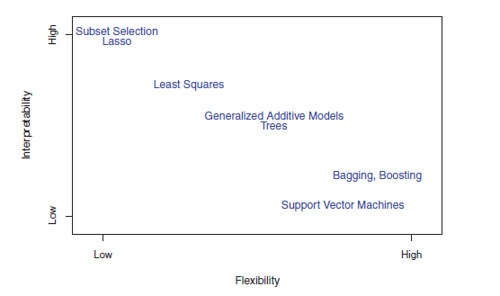
• The lasso, discussed in Chapter 6, relies upon the linear model but uses an alternative fitting procedure for estimating the coefficients ${\beta }_0,{\beta }_1,\cdots ,{\beta }_p$. The new procedure is more restrictive in estimating the coefficients, and sets a number of them to exactly zero. Hence in this sense the lasso is a less flexible approach than linear regression. It is also more interpretable than linear regression, because in the final model the response variable will only be related to a small subset of the predictors — namely, those with non-zero coefficient estimates.
• Generalized additive models (GAMs), discussed in Chapter 7, instead extend the linear model to allow for certain non-linear relationships. Consequently, GAMs are more flexible than linear regression. They are also somewhat less interpretable than linear regression, because the relationship between each predictor and the response is now modeled using a curve.
• Fully non-linear methods such as bagging, boosting, and support vector machines with non-linear kernels, discussed in Chapters 8 and 9, are highly flexible approaches that are harder to interpret.

How to choose models:

• If we are mainly interested in inference, then restrictive models are much more interpretable.
• In some settings where we are only interested in prediction, and the interpretability of the predictive model is simply not of interest, we might expect that it will be best to use the most flexible model available.
• Surprisingly, this is not always the case! We will often obtain more accurate predictions using a less flexible method. This phenomenon, which may seem counterintuitive at first glance, has to do with the potential for overfitting in highly flexible methods.

1.4 Supervised Versus Unsupervised LearningPermalink

P26

1.5 Regression Versus Classification ProblemsPermalink

P28

2.2 Assessing Model AccuracyPermalink

2.1 Measuring the Quality of FitPermalink

In the regression setting, the most commonly-used measure is the Mean Squared Error (MSE)

where $\hat{f}(x_i)$ is the prediction that $\hat{f}$ gives for the i^th observation.

The MSE is computed using the training data that was used to fit the model, and so should more accurately be referred to as the training MSE.

The test MSE, or average squared prediction error is measured on test observations. We’d like to select the model for which the test MSE is as small as possible.

As model flexibility increases, training MSE will decrease, but the test MSE may not. When a given method yields a small training MSE but a large test MSE, we are said to be overfitting the data.

Overfitting refers specifically to the case in which a less flexible model would have yielded a smaller test MSE.

2.2 The Bias-Variance Trade-OffPermalink

The expected test MSE, for a given value $x_0$, can always be decomposed into the sum of three fundamental quantities:

• the variance of $\hat{f}(x_0)$
• the squared bias of $\hat{f}(x_0)$
• and the variance of the error terms $ϵ$

That is,

从 Ng 的课上得知：

• underfitting => high bias
• overfitting => high variance

Equation $(\text{2.2})$ tells us that in order to minimize the expected test error, we need to select a statistical learning method that simultaneously achieves low variance and low bias. Note that variance is inherently a nonnegative quantity, and squared bias is also nonnegative. Hence, we see that the expected test MSE can never lie below $Var(ϵ)$, the irreducible error.

If a method has high variance then small changes in the training data can result in large changes in $\hat{f}$.

On the other hand, bias refers to the error that is introduced by approximating a real-life problem, which may be extremely complicated, by a much simpler model. For example, linear regression assumes that there is a linear relationship between $Y$ and $X_1,X_2,\cdots ,X_p$. It is unlikely that any real-life problem truly has such a simple linear relationship, and so performing linear regression will undoubtedly result in some bias in the estimate of $f$.

Generally, more flexible methods result in less bias.

2.3 The Classification SettingPermalink

P37

Classification 就不用 MSE 来衡量了，改用 training/test error rate

2.3.1 The Bayes ClassifierPermalink

P37

The Bayes Classifier is a very simple classifier that assigns each observation to the most likely class, given its predictor values. In other words, we should simply assign a test observation with predictor vector $x_0$ to the class $j$ for which $Pr(Y=j|X=x_0)$ is largest.

The Bayes classifier produces the lowest possible test error rate, called the Bayes error rate. The Bayes error rate is analogous to the irreducible error, discussed earlier.

2.3.2 K-Nearest NeighborsPermalink

E.g. we have plotted a small training data set consisting of six blue and six orange observations. Our goal is to make a prediction for the point labeled by the black cross. Suppose that we choose $K=3$. Then KNN will first identify the three observations that are closest to the cross. This neighborhood is shown as a circle. It consists of two blue points and one orange point, resulting in estimated probabilities of 2/3 for the blue class and 1/3 for the orange class. Hence KNN will predict that the black cross belongs to the blue class.

Despite the fact that it is a very simple approach, KNN can often produce classifiers that are surprisingly close to the optimal Bayes classifier.

$K$ too small:

• overly flexible
• low bias but very high variance

$K$ too large:

• less flexible
• a decision boundary that is close to linear
• low variance but high bias

3 Lab: Introduction to RPermalink

只记录了新遇到的 function。

Once the data has been loaded, the fix() function can be used to view it in a spreadsheet like window.

> Auto=read.csv (" Auto.csv", header =T,na.strings ="?")
> fix(Auto)

Once the data are loaded correctly, we can use names() to check the variable names.

> names(Auto)
[1] "mpg " "cylinders " " displacement" "horsepower "
[5] "weight " " acceleration" "year" "origin "
[9] "name"

To refer to a variable, we must type the data set and the variable name joined with a $ symbol. Alternatively, we can use the attach() function in order to tell R to make the variables in this data frame available by name.

> plot(Auto$cylinders , Auto$mpg )

> attach (Auto)
> plot(cylinders , mpg)

The pairs() function creates a scatterplot matrix i.e. a scatterplot for every scatterplot pair of variables for any given data set.

> pairs(Auto)
> pairs(~ mpg + displacement + horsepower + weight + acceleration , Auto)

In conjunction with the plot() function, identify() provides a useful interactive method for identifying the value for a particular variable for points on a plot. We pass in three arguments to identify(): the x-axis variable, the y-axis variable, and the variable whose values we would like to see printed for each point. Then clicking on a given point in the plot will cause R to print the value of the variable of interest. Right-clicking on the plot will exit the identify() function

> plot(horsepower ,mpg)
> identify (horsepower ,mpg ,name)

Before exiting R, we may want to save a record of all of the commands that we typed in the most recent session; this can be accomplished using the savehistory() function. Next time we enter R, we can load that history using the loadhistory() function.