R Generating Random Numbers and Random Sampling

感性复习：如何理解钟形曲线Permalink

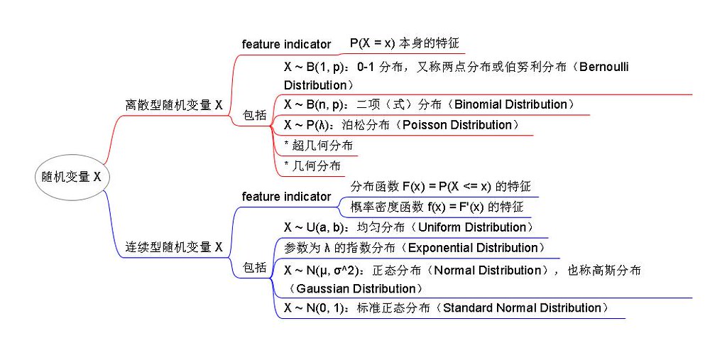
$P(X=x)$ 表示随机变量 $X=x$ 的概率，$F(x)=P(X\le x)$ 称为随机变量 $X$ 的 分布函数。若 $F(x)$ 可微，则 $f(x)=F^{\prime }(x)$ 称为随机变量 $X$ 的 概率密度函数，简称为 概率密度。

$f(x)$ 的值具体是多少没有多大意义，但是 $f(x)$ 值的是大是小可以说明随机变量 $X$ 取值的密集程度，比如 $f(3)>f(2)$，说明 $X=3$ 的样本数多于 $X=2$ 的样本数。

$y=f(x)$ 是 概率密度曲线，$P(x_1<X\le x_2)$ 的值等于 “以 $(x_1,x_2]$ 为底，以 $y=f(x)$ 为顶的曲边梯形的面积”。钟形曲线只是一种特殊的概率密度曲线。

感性复习：分布来分布去Permalink

随机变量 $X$ 有两种大类型：

• 离散型随机变量 $X$
• 连续型随机变量 $X$

对于连续型随机变量 $X$，我们倒腾半天搞出 $F(x)$ 和 $f(x)$ 就是为了描述 $X$ 的特征。那么对于离散型随机变量 $X$ 的特征，我们更多是根据 $P(X=x)$ 这个函数本身的特征来描述。如果 $X$ 具有某些特定的特征，我们称 $X$ 满足某某分布。

新知识：分位数 Quantile [‘kwɒntaɪl]Permalink

对正态分布 $X\sim N(\mu ,{\sigma }^2)$，若 $a<\mu$，有：

• 若 $F(x)=P(X\le x)=a$，称 $x$ 为 下侧 $a$ 分位数（在 $y=f(x)$ 图中 $x=\mu$ 左侧）
• 若 $F(x)=P(X\le x)=1-a$，i.e $P(X>x)=a$，称 $x$ 为 上侧 $a$ 分位数（在 $y=f(x)$ 图中 $x=\mu$ 右侧）

对一个确定的 $a$，它的分位数常写作 $u_a$。比如 $X\sim N(0,1)$ 中，上侧 $u_{0.05}$ = 1.65，则表示 $P(X>1.65)=0.05$。所以你可以把分位数理解为 $X$ 的一种临界值。

正态分布的一些区间特性Permalink

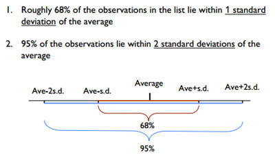
图片来源：Lecture 2: Descriptive Statistics and Exploratory Data Analysis

其实还有，根据 quartile 这一节 IQR 的定义，50% of the observations 是在 [Ave - 0.5*IQR, Ave + 0.5*IQR] 这个区间内的。

正态分布相关函数Permalink

• rnorm: generate random Normal variates with a given mean and standard deviation [ˌdi:viˈeɪʃn]
  • rnorm(n, mean = 0, sd = 1) 即生成 n 个符合正态分布的随机值
  • mean 指 均值，i.e. 期望值，即 $X\sim N(\mu ,{\sigma }^2)$ 中的 $\mu$；默认为 0
  • standard deviation 指 标准差，即 $X\sim N(\mu ,{\sigma }^2)$ 中的 $\sigma$；默认为 1
  • ${\sigma }^2$ 是 方差 variance [ˈvɛriəns]
• dnorm: evaluate the Normal probability density (with a given mean/SD) at a point (or vector of points)
  • dnorm(x, mean = 0, sd = 1, log = FALSE) 计算 $x$ 在这个 N(mean, sd^2) 分布上的概率密度，即 $f(x)$
  • if log = TRUE, probabilities $p$ are given as $\log p$
• pnorm: evaluate the cumulative distribution function for a Normal distribution
  • pnorm(q, mean = 0, sd = 1, lower.tail = TRUE, log.p = FALSE) 计算 q 在这个 N(mean, sd^2) 分布上的分布函数值，即 $F(q)$
  • cumulative distribution 是 累积分布函数，其实就是 F(x)，不知为何我的教材只翻译成分布函数
  • if log.p = TRUE, probabilities $p$ are given as $\log p$
  • if lower.tail = TRUE (default), probabilities are $P[X\le x]$ otherwise, $P[X>x]$.
• qnorm: gives the quantile
  • qnorm(p, mean = 0, sd = 1, lower.tail = TRUE, log.p = FALSE) 给出 $a=p$ 在这个 N(mean, sd^2) 分布上的分位数
  • 默认是给出下侧分位数
  • if lower.tail = FALSE，给出上侧分位数
  • 比如 qnorm(0.05) = -1.644854，qnorm(0.05, lower.tail=F) = 1.644854

泊松分布相关函数Permalink

• rpois: generate random Poisson variates with a given rate
  • rpois(n, lambda) 生成 n 个满足 P(lambda) 泊松分布的随机数
• 同理有 dpois、ppois、qpois

二项分布相关函数Permalink

• rbinom: generate random Binomial variates with a given number of trials and the probability of success on each trial
  • rbinom(n, size, prob) 生成 n 个满足 B(size, prob) 二次分布的随机数
• 同理有 dbinom、pbinom、qbinom

r、d、p、q 一般规律Permalink

• r for random number generation
• d for density, i.e. $f(x)$
• p for cumulative distribution, i.e. $F(x)$
• q for quantile function, i.e. $u_a$

set.seed(n)Permalink

Setting the random number seed with set.seed() ensures reproducibility.

< set.seed(1)
< rnorm(5)
[1] -0.6264538 0.1836433 -0.8356286 1.5952808
[5] 0.3295078
< rnorm(5)
[1] -0.8204684 0.4874291 0.7383247 0.5757814
[5] -0.3053884
< set.seed(1)
< rnorm(5)
[1] -0.6264538 0.1836433 -0.8356286 1.5952808
[5] 0.3295078

set the random number seed when conducting a simulation!

an example of simulating linear modelPermalink

假设 $Y=aX+E$，$X\sim N(0,1)$, $E\sim (0,2^2)$, $a=2$，我们模拟这个曲线可以用：

> set.seed(20)
> x <- rnorm(100)
> e <- rnorm(100, 0, 2)
> y <- 2x + e
> summary(y)
 Min. 1st Qu. Median
-6.4080 -1.5400 0.6789 0.6893 2.9300 6.5050
> plot(x, y)

Random SamplingPermalink

The sample() function draws randomly from a specified set of (scalar) objects allowing you to sample from arbitrary distributions.

> set.seed(1)
> sample(1:10, 4)
[1] 3 4 5 7
> sample(1:10, 4)
[1] 3 9 8 5
> sample(letters, 5)
[1] "q" "b" "e" "x" "p"
> sample(1:10) ## Generate Permutation(序列)
 [1] 4 710 6 9 2 8 3 1 5 
> sample(1:10)
 [1] 2 3 4 1 9 5 10 8 6 7
> sample(1:10, replace = TRUE) ## Sample w/ replacement
 [1] 2 9 7 8 2 8 5 9 7 8