ROC Curve: my interpretation

首先我们来看个例子：

import pandas as pd
import numpy as np
from sklearn.datasets import load_breast_cancer
from sklearn.linear_model import LogisticRegression
from sklearn.metrics import roc_curve

bc = load_breast_cancer()

feat = pd.DataFrame(bc['data'])
feat.columns = bc['feature_names']
label = pd.Series(bc['target'])

train_X = feat.loc[0:99, ]  # contrary to usual python slices, both the start and the stop are included in .loc!
train_y = label.loc[0:99]
test_X = feat.loc[100:, ]
test_y = label.loc[100:]

lr_config = dict(penalty='l2', C=1.0, class_weight=None, random_state=1337,
                 solver='liblinear', max_iter=100, verbose=0, warm_start=False, n_jobs=1)
lr = LogisticRegression(**lr_config)
lr.fit(train_X, train_y)

proba_test_y = lr.predict_proba(test_X)[:, 1]

auroc_df = pd.DataFrame(np.column_stack(roc_curve(test_y, proba_test_y, pos_label=1)))
auroc_df.columns = ["False Positive Rate", "True Positive Rate", "Decision Threshold"]
auroc_df.to_csv("auroc_test.tsv", sep='\t', index=False, header=True)

>>> auroc_df.head(n=3)
	False Positive Rate	True Positive Rate	Decision Threshold
0	0.000000	0.003106	0.999988
1	0.000000	0.624224	0.953624
2	0.006803	0.624224	0.952853
>>> auroc_df.tail(n=3)
	False Positive Rate	True Positive Rate	Decision Threshold
38	0.360544	0.996894	7.970653e-05
39	0.360544	1.000000	7.513310e-05
40	1.000000	1.000000	2.495012e-44

1. Axes

• x-axis 是 $\text{False Positive Rate} = \frac{FP}{TN + FP} = \frac{FP}{N}$
• y-axis 是 $\text{True Positive Rate} = \frac{TP}{TP + FN} = \frac{TP}{P}$

2. 序列规律

我们假设有 $n$ 个 decision thresholds。对每一个 threshold $t_j, j=0,2,\dots,n-1$，我们会计算一个 False Positive Rate $fpr_j$ 和一个 True Positive Rate $tpr_j$。这 $n$ 个点 $(fpr_j, tpr_j)$ 就构成了 ROC curve。

>>> library(ggplot2)
>>> auroc_df <- read.table("auroc_test.tsv", header=TRUE, sep="\t", stringsAsFactors=FALSE)
>>> colnames(auroc_df)
'False.Positive.Rate' 'True.Positive.Rate' 'Decision.Threshold'
>>> p <- ggplot(data=auroc_df, mapping=aes(x=False.Positive.Rate, y=True.Positive.Rate)) + geom_line(size=0.3) + geom_point(size=0.4, color=I("blue"))
>>> p

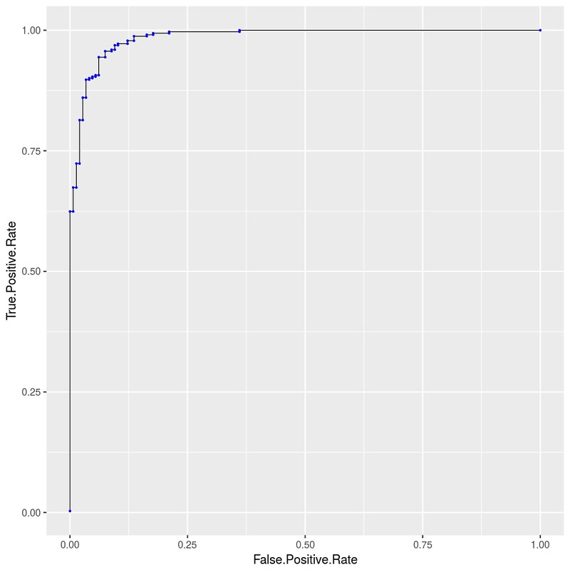
规律：

• $\lbrace fpr_j \rbrace$：从 0 单调递增到 1
• $\lbrace tpr_j \rbrace$：从 0 单调递增到 1
• $\lbrace t_j \rbrace$：从 1 单调递减到 0

所以 ROC curve 第一个点一定是 $(0,0)$，对应 $t_0 = 1$；最后一个点一定是 $(1,1)$，对应 $t_{n-1} = 0$。

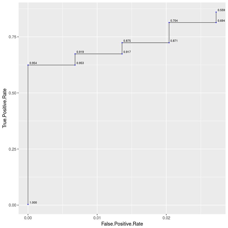
画一个图演示一下 $\lbrace t_j \rbrace$ 单调递减性：

ggplot(data=auroc_df[0:10, ], mapping=aes(x=False.Positive.Rate, y=True.Positive.Rate)) + geom_line(size=0.3) + geom_point(size=0.4, color=I("blue")) + geom_text(aes(label=sprintf("%0.3f", round(Decision.Threshold, digits=3))), hjust=-0.2, vjust=-0.4, size=2.2)

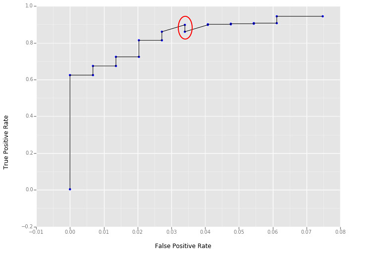
注意用 python 画图时，会出现 $tpr_j > tpr_{j+1}$ 的情况。看上去是违背了单调性。其原因是对 float 处理的误差。比如其实是 $tpr_j = tpr_{j+1} = 0.81366$，但 python 读取后变成了 $tpr_j = 0.81366001 > tpr_{j+1} = 0.81365999$。（此处存疑；参 ggplot2: use geom_line() carefully when your x-axis data are descending）

误差导致的作图如下：

p = ggplot(aesthetics=aes(x="False Positive Rate", y="True Positive Rate"), data=auroc_df.loc[0:20,:]) + geom_line() + geom_point(color="blue")
p

3. 单调性的原因

假设 test dataset 的 ground-true labels 为 $y = \lbrace y_i \rbrace$，examples 为 $X = \lbrace x_i \rbrace$，classifier.predict_proba(X)[:, 1] 得到概率为 $\lbrace p_i \rbrace$，classifier.predict(X) 得到预测为 $\lbrace h(x_i) = (p_i > t) \rbrace$。

当 threshold 从 $t_j$ 变化到 $t_{j+1}$ 时：

• $t_j > t_{j+1}$
• ground-true positive 的数量 $P$ 不变
• ground-true negative 的数量 $N$ 不变
• $\lbrace h(x_i) = 1 \rbrace \subseteq \lbrace h(x_{i+1}) = 1 \rbrace $
  • threshold 减小，predict 为 positive 的数量只多不少
  • 尤其当 $t = 0$ 时，$\vert \lbrace h(x_i) = 1 \rbrace \vert = n$
• 对 $\lbrace fpr_j \rbrace$ 而言:
  • $FP \rvert_{t_j} \leq FP \rvert_{t_{j+1}}$
    • $\lbrace h(x_{i+1}) = 1 \rbrace \setminus \lbrace h(x_i) = 1 \rbrace$ 是新增的 predict 为 positive 的 cases，其中必然有 0 个或者若干个新增的 False Positive
  • $fpr_{j} \leq fpr_{j+1}$
• 对 $\lbrace tpr_j \rbrace$ 而言:
  • $TP \rvert_{t_j} \leq TP \rvert_{t_{j+1}}$
    • $\lbrace h(x_{i+1}) = 1 \rbrace \setminus \lbrace h(x_i) = 1 \rbrace$ 是新增的 predict 为 positive 的 cases，其中必然有 0 个或者若干个新增的 True Positive
  • $tpr_{j} \leq tpr_{j+1}$

4. Randon Guess 与 AUROC = 0.5

有一类描述非常的 misleading，比如 quote from Can AUC-ROC be between 0-0.5：

… a predictor which makes random guesses has an AUC-ROC score of 0.5.

主要原因是这里 random guess 往往是忽视 thresholds 的，它和 thresholds 没有关系，所以本质上 a predictor which makes random guess 是做不出 ROC curve 的，它只有一个 $(fpr, tpr)$ 点，无法构成连线。举个例子：quote from Advantages of AUC vs standard accuracy：

Similarly, if you predict a random assortment of 0’s and 1’s, let’s say 90% 1’s, you could get the point (0.9, 0.9), which again falls along that diagonal line.

这里需要这样理解：

• 你在 $P$ 上预测了 90% 为 Positive，这些全部都是 True Positive，所以 $TP = 0.9 * P$
• 你在 $N$ 上预测了 90% 为 Positive，这些全部都是 False Positive，所以 $FP = 0.9 * N$

所以 AUROC = 0.5 这条线本质上是一系列 predictors which make random guess，不可能是某个特定的 predictor

5. 可能出现 AUROC < 0.5 吗？为什么我们常见的 AUROC 都是 > 0.5？

AUROC 的范围是 [0, 1]，所以当然可能会有 AUROC < 0.5。我们先来研究一下为什么常见的 AUROC 都是 > 0.5。

这个要借鉴 wikipedia: Receiver operating characteristic 上 $tpr$ 和 $fpr$ 高级的积分 representation：

In binary classification, the class prediction for each instance is often made based on a continuous random variable $X$, which is a “score” computed for the instance (e.g. estimated probability in logistic regression). Given a threshold parameter $T$, the instance is classified as “positive” if $X>T$, and “negative” otherwise. $X$ follows a probability density $f_{1}(x)$ if the instance actually belongs to class “positive”, and $f_{0}(x)$ if otherwise. Therefore, the true positive rate is given by $\operatorname{TPR}(T)=\int_{T}^{\infty}f_{1}(x)\,dx$ and the false positive rate is given by $\operatorname{FPR}(T)=\int_{T}^{\infty}f_{0}(x)\,dx$.

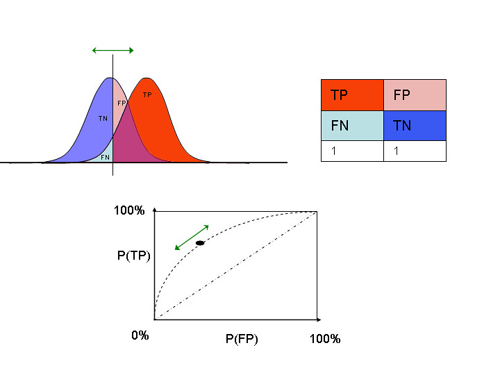
用我们自己的符号表示就是：

• $tpr_j=\int_{t_j}^{1}f_{1}(p)\,dp$
• $fpr_j=\int_{t_j}^{1}f_{0}(p)\,dp$

中间的 vertical bar 是 threshold $t_j$，threshold 右边 $f_1$ bell 的面积就是 $tpr_j$，threshold 右边 $f_0$ bell 的面积则是 $fpr_j$。一般情况下，$f_1$ bell 比 $f_0$ bell 靠右，所以：

• 如果 $t_j = 0$，则 $t_j$ 右边 $f_1$ bell 的面积和 $f_0$ bell 的面积都是 1
• 如果 $t_j = 1$，则 $t_j$ 右边 $f_1$ bell 的面积和 $f_0$ bell 的面积都是 0
• otherwise，则 $t_j$ 右边 $f_1$ bell 的面积永远大于 $f_0$ bell 的面积，因为 $f_1$ bell 更靠右

所以这种情况下永远有 $tpr_j \ge fpr_j$。

那么问题来了：为什么 $f_1$ bell 会比 $f_0$ bell 靠右？因为通常情况下我们取的 $P$ 是 classifier.predict_proba(X)[:, 1]，必然有 $\operatorname{mean}( \lbrace p_i \rvert_{x_i \text{ is positive}} \rbrace ) \ge \operatorname{mean}( \lbrace p_i \rvert_{x_i \text{ is negative}} \rbrace )$。这也就解释了为什么通常情况下 AUROC 都是 > 0.5。

同理，想要 AUROC < 0.5，你设法把 $f_0$ bell 移到 $f_1$ bell 右边就可以了。最简答的做法就是：取 $P$ 为 classifier.predict_proba(X)[:, 0]；站在 predict 的角度，这么做相当于 flip the prediction。所以你算出了 AUROC < 0.5 也不要慌，换一下 label 就正常了。

再衍生一下：如果 $f_1$ bell 和 $f_0$ bell 重合，说明什么？说明你的 $\lbrace p_i \rvert_{x_i \text{ is positive}} \rbrace$ 和 $\lbrace p_i \rvert_{x_i \text{ is negative}} \rbrace$ 没有区分度，满足这一条件的 predicitor 是更广泛意义上的 random guess，前面 “90% 1’s” 这样的 predictor 只能算是这种情况的特例。

6. 为什么说 AUROC 比 accuracy 好？

主要就好在 accuracy 识别不了 random guess。比如 90% $P$ 和 10% $N$ 的数据集，random guess 是 “always 1”，这样 accuracy 也能有 90%。

7. 为什么有人说 you should not use ROC curve with highly imbalance data？

这样的言论比比皆是，比如 Credit Card Fraud: Handling highly imbalance classes and why Receiver Operating Characteristics Curve (ROC Curve) should not be used, and Precision/Recall curve should be preferred in highly imbalanced situations。

我的觉得有点言重了，但是 ROC 的不足的确是存在的。

更好地讨论这个问题的一篇文章是 The Precision-Recall Plot Is More Informative than the ROC Plot When Evaluating Binary Classifiers on Imbalanced Datasets。

ROC 在处理 imbalanced data 时的不足是：False Positive Rate 不足以反映 $FP$ 的数量。这篇文章的例子（Section Results and Discussion）：

• 考虑最常见的 $N > P$ 的情况
• Balanced dataset: $P=1000, N=1000$; classifier $A$ predicts at threashold $t$: $TP=500, FP=160$
• Imbalanced dataset: $P=1000, N=10000$; classifier $B$ predicts at the same threashold $t$: $TP=500, FP=1600$

如果在所有的 theashold 上都有这样类似的关系，i.e. $TP_A = TP_B, FP_A = \frac{1}{10} FP_B$，那么这两个 classifiers 的 ROC 是完全一样的，但是 classifier $B$ 的 $FP > TP$ 让人很难接受。简单概括一下这种情况就是：imbalanced dataset 上 performance 不好，但是 ROC 看不出来。

那如果是 $N < P$ 的情况呢？仿照上面例子的情形，可以简单概括为：imbalanced dataset 上 performance 更好，但是 ROC 看不出来。

还有一种说法也比较恰当：ROC is not sensitive to class balance。

待续：更复杂的积分形式

复习一下符号：假设 $\operatorname f(x) = \frac{1}{2} x^2$，那么 $\operatorname f’(x) = x$。一般有 $\operatorname f(x) = \int \operatorname f’(x) dx$，$\operatorname f’ = \frac{df}{dx}$。算 $\operatorname f’$ 的面积则是 $A = \int_{a}^{b} \operatorname f’(x) dx = \operatorname f(x) \rvert_{a}^{b}$

wikipedia: Receiver operating characteristic 上的这个式子我推不出来：

\[\begin{aligned} A &=\int_{\infty}^{-\infty} \operatorname{TPR}(T) (- \operatorname{FPR}'(T))\,dT \newline &=\int_{-\infty}^{\infty} \int_{-\infty}^{\infty} \operatorname I(T'>T)f_{1}(T') \operatorname f_{0}(T)\,dT'\,dT \newline &=\operatorname P(X_{1}>X_{0}) \end{aligned}\]

到底是 $dT$ 还是 $dp$ 很容易混淆，有需要的时候再研究

更新：等价形式

The meaning and use of the area under a receiver operating characteristic (ROC) curve 是篇很好的文章。它提到：这 3 种 metrics 是等价的：

1. “True” AUROC
   • “True” 的意思是 sample 数要够多，有限的 sample 数不能代表 population，只能算是 estimate
2. $\operatorname P(X_{1}>X_{0})$ （即上面 wikipedia 的那个大积分形式）
   • where $X_{1}$ is the score for a positive instance and $X_{0}$ is the score for a negative instance
   • That is to say, AUROC is equal to the probability that a classifier will rank a randomly chosen positive instance higher than a randomly chosen negative one (assuming ‘positive’ ranks higher than ‘negative’)
   • 这个积分的证明在文章的 reference [6] Green D, Swets J. Signal detection theory and psychophysics. New York: John Wiley and Sons, 1966: 45-49 里。（原书我找不到，目前看来只能去买了……）
3. Wilcoxon statistic (as in Wilcoxon-Mann-Whitney test)