Probability

总结自 Coursera lecture Statistical Inference section 02 Probability。

---

1. Notation

Symbol	Definition	Example
$\Omega$	The sample space, the collection of possible outcomes of an experiment	Die roll, $\Omega = \lbrace 1,2,3,4,5,6 \rbrace$
$E$	An event, a subset of sample space	Die roll is even, $E = \lbrace 2,4,6 \rbrace$
$\omega$	An elementary or simple event, a particular result of an experiment	Die roll is a four, $\omega = 4$
$\phi$	The null event or the empty set

2. Interpretation of set operations

1.$\omega \in E$ implies that $E$ occurs when$\omega$occurs 2.$\omega \notin E$ implies that $E$ does not occur when $\omega$ occurs 3.$E \subset F$ implies that the occurrence of $E$ implies the occurrence of $F$ 4.$E \cap F$ implies the event that both $E$ and $F$ occur 5.$E \cup F$ implies the event that at least one of $E$ or $F$ occur 6.$E \cap F = \phi$ means that $E$ and $F$ are mutually exclusive, or cannot both occur 7.$E^c$ or $\bar{E}$ is the event that $E$ does not occur

3. Probability

A probability measure, $P$, is a function from the collection of possible events so that the following hold:

1. For an event $E \subset \Omega$, $0 \leq P(E) \leq 1$

2. $P(\Omega) = 1$

3. If $E_1$ and $E_2$ are mutually exclusive events, $P(E_1 \cup E_2) = P(E_1) + P(E_2)$.

Part 3 of the definition implies finite additivity: $P(\bigcup_{i=1}^{n} A_i) = \sum_{i=1}^n P(A_i)$, where the $A_i$ are mutually exclusive.

4. Consequences (推论)

• $P(\phi) = 0$

• $P(E) = 1 - P(E^c)$

• If $A \subset B$, then $P(A) \leq P(B)$

• $P(A \cup B) = P(A) + P(B) - P(A \cap B) = 1 - P(A^c \cap B^c)$

• $P(A \cap B^c) = P(A) - P(A \cap B)$

• $P(\bigcup_{i=1}^{n} E_i) \leq \sum_{i=1}^n P(E_i)$

• $P(\bigcup_{i=1}^{n} E_i) \geq max(P(E_i))$

5. Random variables

• A random variable is a numerical outcome of an experiment.
• 2 varieties
  • Discrete
  • Continuous
• Discrete random variable are random variables that take on only a countable number of possibilities.

  • $P(X = k)$

  • described by PMF
• Continuous random variable can take any value on the real line or some subset of the real line.

  • $P(X \in A)$

  • discribed by PDF and CDF

6. PMF: Probability Mass Function

A PMF evaluated at a value corresponds to the probability that a random variable takes that value (我觉得你可以理解为 $p(x) = P(X = x)$).

To be a valid PMF, $p$ must satisfy:

1.$p(x) \geq 0$ for all $x$ 2.$\sum_{x} p(x) = 1$ (The sum is taken over all of the possible values for $x$)

E.g., let $X$ be the result of a coin flip where $X=0$ represents tails and $X=1$ represents heads. Suppose that we do not know whether or not the coin is fair. Let $\theta$ be the probability of a head expressed as a proportion (between 0 and 1). Then we get:

\[p(x) = \theta^x (1 - \theta)^{1-x},\, \text{for x = 0,1}\]

PMF 其实就是分布律，用来描述 discrete random variable

7. PDF: Probability Density Function

A PDF, is a function associated with a continuous random variable.

Areas under the PDF correspond to probabilities for that random variable.

To be a valid PDF, $f$ must satisfy:

1.$f(x) \geq 0$ for all $x$

1. The area under $f(x)$ is 1

实际有：$P [a \le X \le b] = \int_a^b f(x) \, dx$

8. CDF: Cumulative Distribution Function & SF: Survival Function

The CDF of a random variable $X$ is defined as the function:

\[F(x) = P(X \leq x)\]

This definition applies regardless of whether is discrete or continuous.

The SF of a random variable $X$ is defined as:

\[S(x) = P(X > x)\]

Notice that $S(x) = 1 - F(x)$

For continuous random variables, the PDF is the derivative of the CDF, i.e. $f(x) = F’(x)$

9. Example: Beta Distribution

More details in wikipedia Beta distribution.

If $x \in [0, 1]$ and $X \sim Beta(\alpha,\beta)$, 我们称 $X$ 足 $\alpha, \beta$ 控制的 beta 分布。$\alpha, \beta > 0$ and are both real number, a.k.a “shape parameters”.

PDF is defined as $f(x \vert \alpha,\beta) = \frac{x^{\alpha-1} (1-x)^{\beta-1}}{B(\alpha, \beta)}$

where constant $B(\alpha, \beta) = \int_{0}^{1} t^{\alpha-1} (1-t)^{\beta-1} dt$

or with Gamma Funtion $\Gamma(n) = \begin{cases} (n-1)! & \text { n is a positive integer } \newline \int_{0}^{1} t^{\alpha-1} (1-t)^{\beta-1} dt & \text { n is real or complex } \end{cases}$

we can rewrite $B(\alpha, \beta) = \frac{\Gamma(\alpha) \Gamma(\beta)}{\Gamma(\alpha + \beta)}$

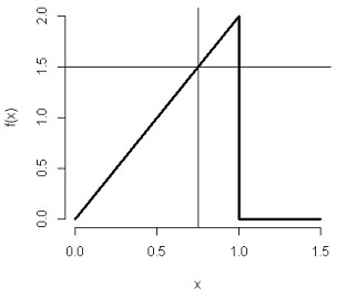
If $\alpha = 2$ and $\beta = 1$, then $B(\alpha, \beta) = \frac{1!\times0!}{2!} = 0.5$ or $B(\alpha, \beta) = \int_{0}^{1} t \cdot dt = \frac{1}{2}t^2 \vert _{0}^{1} = 0.5$, therefore $f(x) = 2x$ and $F(x) = x^2$.

我们在 R 中执行 pbeta(0.75, 2, 1) 会得到 0.5625。根据 R Generating Random Numbers and Random Sampling 里总结的规律，p 开头的都是求 CDF，i.e. $F(x)$，所以这里 pbeta(0.75, 2, 1) 的意义就是：当 $\alpha = 2$ and $\beta = 1$ 时，求 $F(0.75)$。最终得到 $F(0.75) = 0.5625$。这和我们用 $f(x)$ 的面积来算的结果是一致的：

> x <- c(0, 1, 1, 1.5)
> y <- c(0, 2, 0, 0)
> plot(x, y, lwd = 3, frame = FALSE, type = "l", ylab="f(x)")
> abline(h=1.5, v=0.75)

\[F(0.75) = \frac{1.5 \times 0.75}{2} = 0.5625\]