Asymptotics: The Law of Large Numbers and The Central Limit Theorem
总结自 Coursera lecture Statistical Inference section 07 Asymptotics。新的 slide 省略了部分推导过程,最好同时参考下旧的 slide。
0. Asymptotics
Asymptotics,[æsɪmp’tɒtɪks] 渐近性,其实就是讲 $\text{number of trials} \rightarrow + \infty$ 时的一些性质。
1. The Law of Large Numbers
1.1 Definition
There are many variations on the LLN; we are using a particularly lazy version here.
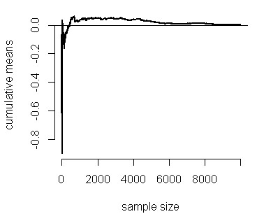
The law of large numbers states that if $X_1,\ldots X_n$ are i.i.d. from a population with mean $\mu$ and variance $\sigma^2$, then $\overline{X}$, the sample average of the n observations, converges in probability to $\mu$, i.e.
\[\begin{align} \overline{X}=\frac{1}{n}(X_1+\cdots+X_n) \newline \overline{X} \to \mu \text{ when } n \to \infty \end{align}\]Or more generally, the average of the results obtained from a large number of trials (i.e. n, since we get an observation per trial) should be close to the expected value, and will tend to become closer as more trials are performed.
1.2 Simulation
n <- 10000;
means <- cumsum(rnorm(n)) / (1:n) ## cumsum 累积求和,e.g. cumsum(c(1,2,3)) = c(1,3,6)
plot(1:n, means, type = "l", lwd = 2, frame = FALSE, ylab = "cumulative means", xlab = "sample size")
abline(h = 0)

1.3 Consistency and Bias of an estimator
- An estimator is consistent if it converges to what you want to estimate, i.e. $\hat{X} \to X$
- Consistency is neither necessary nor sufficient for one estimator to be better than another
- The LLN basically states that the sample mean is consistent
- The sample variance and the sample standard deviation are consistent as well
- An estimator is unbiased if the expected value of an estimator is what its trying to estimate, i.e. $E[\hat{X}] = X$
- The sample mean is unbiased
- The sample variance is unbiased
- The sample standard deviation is biased (complicated proof. see Why is sample standard deviation a biased estimator of σ)
2. The Central Limit Theorem
2.1 Definition
CLT says
\[\overline{X} \to \sim \mbox{N}(\mu, \frac{\sigma^2}{n}) \text{ when } n \to \infty\]In another word
\[\begin{align} \frac{\overline X - \mu}{\sigma / \sqrt{n}} &= \frac{\mbox{Estimate} - \mbox{Mean of estimate}}{\mbox{Std. Err. of estimate}} \newline & \to \sim \mbox{N}(0,1) \text{ when } n \to \infty \end{align}\]2.2 Confidence intervals
置信区间只在频率统计中使用。在贝叶斯统计中的对应概念是可信区间。
举例来说,如果在一次大选中某人的支持率为 55%,而置信水平 0.95 上的置信区间是(50%, 60%),那么他的真实支持率有 95% 的机率落在 50% 和 60% 之间,因此他的真实支持率不足一半的可能性小于 2.5%(假设分布是对称的)。
$[\overline{X} - \frac{2\sigma}{\sqrt n}, \overline{X} + \frac{2\sigma}{\sqrt n}]$ is called a 95% interval for $\mu$.
更多内容可以参考 Stat Trek: What is a Confidence Interval?。
2.3 Apply CLT to Bernoulli estimators
\[\begin{align} \because \sigma^2 &= p(1 - p) \newline \therefore \frac{2\sigma}{\sqrt n} &= 2 \sqrt{\frac{p(1 - p)}{n}} \newline \because p(1-p) &\leq \frac{1}{4}, \text{for}\, 0 \leq p \leq 1 \newline \therefore \frac{2\sigma}{\sqrt n} &= 2 \sqrt{\frac{p(1 - p)}{n}} \leq 2 \sqrt{\frac{1}{4n}} = \frac{1}{\sqrt{n}} \end{align}\]$\therefore \overline X \pm \frac{1}{\sqrt{n}}$ is a quick CI estimate for $p$ (since $\mu = p$ in Bernoulli)
Exercise I
What is the probability of getting 45 or fewer heads out 100 flips of a fair coin? (Use the CLT, not the exact binomial calculation)
- $\mu = p = 0.5$
- $\sigma^2 = p*(1-p) = 0.25, \frac{\sigma}{\sqrt{100}} = 0.05$
- $\overline X = \frac{45}{100} = 0.45$
pnorm(0.45, mean=0.5, sd=0.05)
## [1] 0.1586553
Exercise II
Your campaign advisor told you that in a random sample of 100 likely voters, 56 intent to vote for you. Can you relax? Do you have this race in the bag?
- $\overline X = \frac{56}{100} = 0.56$
- $\frac{1}{\sqrt{100}} = 0.1$
- an approximate 95% interval of p is [0.46, 0.66]
- Not enough for you to relax, better go do more campaigning!
2.4 Calculate Poisson interval with R
A nuclear pump failed 5 times out of 94.32 days, give a 95% confidence interval for the failure rate per day (i.e. $\lambda$)?
poisson.test(x, T = 94.32)$conf
## [1] 0.01721 0.12371
## attr(,"conf.level")
## [1] 0.95
留下评论